Ecosyste.ms: Awesome
An open API service indexing awesome lists of open source software.
https://github.com/probml/dynamax
State Space Models library in JAX
https://github.com/probml/dynamax
hidden-markov-models jax kalman-filter python state-space-models
Last synced: 4 days ago
JSON representation
State Space Models library in JAX
- Host: GitHub
- URL: https://github.com/probml/dynamax
- Owner: probml
- License: mit
- Created: 2022-04-11T23:42:29.000Z (about 2 years ago)
- Default Branch: main
- Last Pushed: 2024-05-08T20:06:25.000Z (about 1 month ago)
- Last Synced: 2024-06-12T21:14:37.915Z (10 days ago)
- Topics: hidden-markov-models, jax, kalman-filter, python, state-space-models
- Language: Jupyter Notebook
- Homepage: https://probml.github.io/dynamax/
- Size: 190 MB
- Stars: 624
- Watchers: 24
- Forks: 65
- Open Issues: 53
-
Metadata Files:
- Readme: README.md
- Contributing: CONTRIBUTING.md
- License: LICENSE
Lists
- awesome-stars - dynamax
README
# Welcome to DYNAMAX!


Dynamax is a library for probabilistic state space models (SSMs) written
in [JAX](https://github.com/google/jax). It has code for inference
(state estimation) and learning (parameter estimation) in a variety of
SSMs, including:
- Hidden Markov Models (HMMs)
- Linear Gaussian State Space Models (aka Linear Dynamical Systems)
- Nonlinear Gaussian State Space Models
- Generalized Gaussian State Space Models (with non-Gaussian emission
models)
The library consists of a set of core, functionally pure, low-level
inference algorithms, as well as a set of model classes which provide a
more user-friendly, object-oriented interface. It is compatible with
other libraries in the JAX ecosystem, such as
[optax](https://github.com/deepmind/optax) (used for estimating
parameters using stochastic gradient descent), and
[Blackjax](https://github.com/blackjax-devs/blackjax) (used for
computing the parameter posterior using Hamiltonian Monte Carlo (HMC) or
sequential Monte Carlo (SMC)).
## Documentation
For tutorials and API documentation, see: https://probml.github.io/dynamax/.
For an extension of dynamax that supports structural time series models,
see https://github.com/probml/sts-jax.
For an illustration of how to use dynamax inside of [bayeux](https://jax-ml.github.io/bayeux/) to perform Bayesian inference
for the parameters of an SSM, see https://jax-ml.github.io/bayeux/examples/dynamax_and_bayeux/.
## Installation and Testing
To install the latest releast of dynamax from PyPi:
``` {.console}
pip install dynamax # Install dynamax and core dependencies, or
pip install dynamax[notebooks] # Install with demo notebook dependencies
```
To install the latest development branch:
``` {.console}
pip install git+https://github.com/probml/dynamax.git
```
Finally, if you\'re a developer, you can install dynamax along with the
test and documentation dependencies with:
``` {.console}
git clone [email protected]:probml/dynamax.git
cd dynamax
pip install -e '.[dev]'
```
To run the tests:
``` {.console}
pytest dynamax # Run all tests
pytest dynamax/hmm/inference_test.py # Run a specific test
pytest -k lgssm # Run tests with lgssm in the name
```
## What are state space models?
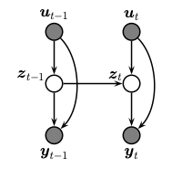
A state space model or SSM is a partially observed Markov model, in
which the hidden state, $z_t$, evolves over time according to a Markov
process, possibly conditional on external inputs / controls /
covariates, $u_t$, and generates an observation, $y_t$. This is
illustrated in the graphical model below.
The corresponding joint distribution has the following form (in dynamax,
we restrict attention to discrete time systems):
$$p(y_{1:T}, z_{1:T} | u_{1:T}) = p(z_1 | u_1) p(y_1 | z_1, u_1) \prod_{t=1}^T p(z_t | z_{t-1}, u_t) p(y_t | z_t, u_t)$$
Here $p(z_t | z_{t-1}, u_t)$ is called the transition or dynamics model,
and $p(y_t | z_{t}, u_t)$ is called the observation or emission model.
In both cases, the inputs $u_t$ are optional; furthermore, the
observation model may have auto-regressive dependencies, in which case
we write $p(y_t | z_{t}, u_t, y_{1:t-1})$.
We assume that we see the observations $y_{1:T}$, and want to infer the
hidden states, either using online filtering (i.e., computing
$p(z_t|y_{1:t})$ ) or offline smoothing (i.e., computing
$p(z_t|y_{1:T})$ ). We may also be interested in predicting future
states, $p(z_{t+h}|y_{1:t})$, or future observations,
$p(y_{t+h}|y_{1:t})$, where h is the forecast horizon. (Note that by
using a hidden state to represent the past observations, the model can
have \"infinite\" memory, unlike a standard auto-regressive model.) All
of these computations can be done efficiently using our library, as we
discuss below. In addition, we can estimate the parameters of the
transition and emission models, as we discuss below.
More information can be found in these books:
> - \"Machine Learning: Advanced Topics\", K. Murphy, MIT Press 2023.
> Available at .
> - \"Bayesian Filtering and Smoothing, Second Edition\", S. Särkkä and L. Svensson, Cambridge
> University Press, 2023. Available at
>
## Example usage
Dynamax includes classes for many kinds of SSM. You can use these models
to simulate data, and you can fit the models using standard learning
algorithms like expectation-maximization (EM) and stochastic gradient
descent (SGD). Below we illustrate the high level (object-oriented) API
for the case of an HMM with Gaussian emissions. (See [this
notebook](https://github.com/probml/dynamax/blob/main/docs/notebooks/hmm/gaussian_hmm.ipynb)
for a runnable version of this code.)
```python
import jax.numpy as jnp
import jax.random as jr
import matplotlib.pyplot as plt
from dynamax.hidden_markov_model import GaussianHMM
key1, key2, key3 = jr.split(jr.PRNGKey(0), 3)
num_states = 3
emission_dim = 2
num_timesteps = 1000
# Make a Gaussian HMM and sample data from it
hmm = GaussianHMM(num_states, emission_dim)
true_params, _ = hmm.initialize(key1)
true_states, emissions = hmm.sample(true_params, key2, num_timesteps)
# Make a new Gaussian HMM and fit it with EM
params, props = hmm.initialize(key3, method="kmeans", emissions=emissions)
params, lls = hmm.fit_em(params, props, emissions, num_iters=20)
# Plot the marginal log probs across EM iterations
plt.plot(lls)
plt.xlabel("EM iterations")
plt.ylabel("marginal log prob.")
# Use fitted model for posterior inference
post = hmm.smoother(params, emissions)
print(post.smoothed_probs.shape) # (1000, 3)
```
JAX allows you to easily vectorize these operations with `vmap`.
For example, you can sample and fit to a batch of emissions as shown below.
```python
from functools import partial
from jax import vmap
num_seq = 200
batch_true_states, batch_emissions = \
vmap(partial(hmm.sample, true_params, num_timesteps=num_timesteps))(
jr.split(key2, num_seq))
print(batch_true_states.shape, batch_emissions.shape) # (200,1000) and (200,1000,2)
# Make a new Gaussian HMM and fit it with EM
params, props = hmm.initialize(key3, method="kmeans", emissions=batch_emissions)
params, lls = hmm.fit_em(params, props, batch_emissions, num_iters=20)
```
These examples demonstrate the dynamax models, but we can also call the low-level
inference code directly.
## Contributing
Please see [this page](https://github.com/probml/dynamax/blob/main/CONTRIBUTING.md) for details
on how to contribute.
## About
Core team: Peter Chang, Giles Harper-Donnelly, Aleyna Kara, Xinglong Li, Scott Linderman, Kevin Murphy.
Other contributors: Adrien Corenflos, Elizabeth DuPre, Gerardo Duran-Martin, Colin Schlager, Libby Zhang and other people [listed here](https://github.com/probml/dynamax/graphs/contributors)
MIT License. 2022