Ecosyste.ms: Awesome
An open API service indexing awesome lists of open source software.
https://github.com/JoGall/soccermatics
Tools for visualisation and analysis of soccer tracking and event data
https://github.com/JoGall/soccermatics
Last synced: 3 months ago
JSON representation
Tools for visualisation and analysis of soccer tracking and event data
- Host: GitHub
- URL: https://github.com/JoGall/soccermatics
- Owner: JoGall
- Created: 2017-01-19T14:37:08.000Z (over 7 years ago)
- Default Branch: master
- Last Pushed: 2021-08-09T11:56:01.000Z (almost 3 years ago)
- Last Synced: 2024-02-03T11:04:03.218Z (5 months ago)
- Language: R
- Homepage:
- Size: 101 MB
- Stars: 296
- Watchers: 30
- Forks: 36
- Open Issues: 9
-
Metadata Files:
- Readme: README.md
Lists
- awesome-r-dataviz - soccermatics - Tools for visualisation and analysis of soccer tracking and event data. (ggplot / Domain-specific)
- awesome-soccer-analytics - soccermatics - (R) Tools for visualisation and analysis of soccer spatiotemporal data. (Open Source Libraries / Visualisation)
- awesome-stars - JoGall/soccermatics - Tools for visualisation and analysis of soccer tracking and event data (R)
README
soccermatics
=====
soccermatics provides tools to visualise spatial tracking and event data from football (soccer) matches. There are currently functions to visualise shot maps (with xG), average positions, heatmaps, and individual player trajectories. There are also helper functions to smooth, interpolate, and prepare x,y-coordinate tracking data for plotting and calculating further metrics.
Many more functions are planned - see [To Do List](https://github.com/JoGall/soccermatics/issues/8) - suggestions and/or help welcomed!
The sample x,y-coordinate tracking data in `tromso` and `tromso_extra` were made available by [Pettersen et al. (2014)](http://home.ifi.uio.no/paalh/dataset/alfheim/), whilst the event data in `statsbomb` is taken from the World Cup 2018 data [made public by StatsBomb](https://github.com/statsbomb/open-data).
Use of the name soccermatics kindly permitted by the eponymous book's author, [David Sumpter](https://www.bloomsbury.com/uk/soccermatics-9781472924124/).
soccermatics is built on R v3.4.2.
---
### Installation
You can install `soccermatics` from GitHub in R using [`devtools`](https://github.com/hadley/devtools):
```{r}
if (!require("devtools")) install.packages("devtools")
devtools::install_github("jogall/soccermatics")
library(soccermatics)
```
---
### Examples
Below are some sample visualisations produced by `soccermetrics` with code snippets underneath. See the individual help files for each function (e.g. `?soccerHeatmap`) for more information.
#### Shotmaps (showing xG)
Dark theme:
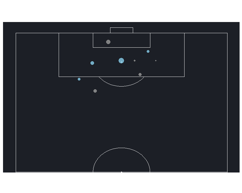
```{r}
statsbomb %>%
filter(team.name == "France") %>%
soccerShotmap(theme = "dark")
```
Grass theme with custom colours:

```{r}
statsbomb %>%
filter(team.name == "Argentina") %>%
soccerShotmap(theme = "grass", colGoal = "yellow", colMiss = "blue", legend = T)
```
#### Passing networks
Default aesthetics:

```{r}
statsbomb %>%
filter(team.name == "Argentina") %>%
soccerPassmap(fill = "lightblue", arrow = "r",
title = "Argentina (vs France, 30th June 2018)")
```
Grass background, non-transparent edges:

```{r}
statsbomb %>%
filter(team.name == "France") %>%
soccerPassmap(fill = "blue", minPass = 3,
edge_max_width = 30, edge_col = "grey40", edge_alpha = 1,
title = "France (vs Argentina, 30th June 2018)")
```
#### Heatmaps
Passing heatmap with approx 10x10m bins:
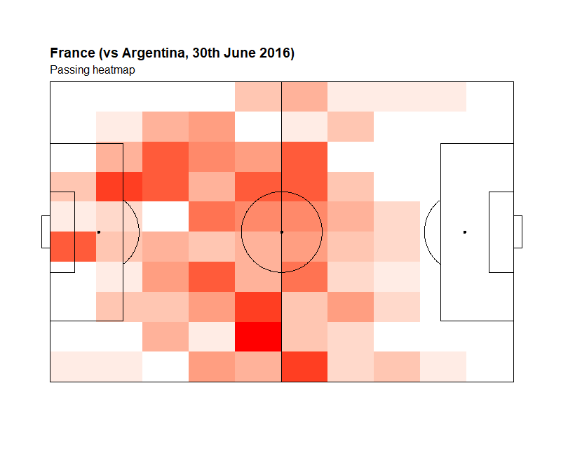
```{r}
statsbomb %>%
filter(type.name == "Pass" & team.name == "France") %>%
soccerHeatmap(x = "location.x", y = "location.y",
title = "France (vs Argentina, 30th June 2016)",
subtitle = "Passing heatmap")
```
Defensive pressure heatmap with approx 5x5m bins:

```{r}
statsbomb %>%
filter(type.name == "Pressure" & team.name == "France") %>%
soccerHeatmap(x = "location.x", y = "location.y", xBins = 21, yBins = 14,
title = "France (vs Argentina, 30th June 2016)",
subtitle = "Defensive pressure heatmap")
```
Player position heatmaps also possible using TRACAB-style x,y-location data.
#### Average position
Average pass position:

```{r}
statsbomb %>%
filter(type.name == "Pass" & team.name == "France" & minute < 43) %>%
soccerPositionMap(id = "player.name", x = "location.x", y = "location.y",
fill1 = "blue", grass = T,
arrow = "r",
title = "France (vs Argentina, 30th June 2016)",
subtitle = "Average pass position (1' - 42')")
```
Average pass position (both teams):

```{r}
statsbomb %>%
filter(type.name == "Pass" & minute < 43) %>%
soccerPositionMap(id = "player.name", team = "team.name", x = "location.x", y = "location.y",
fill1 = "lightblue", fill2 = "blue", label_col = "black",
repel = T, teamToFlip = 2,
title = "France vs Argentina, 30th June 2018",
subtitle = "Average pass position (1' - 42')")
```
Average player position using TRACAB-style x,y-location data:

```{r}
tromso_extra[1:11,] %>%
soccerPositionMap(grass = T, title = "Tromsø IL (vs. Strømsgodset, 3rd Nov 2013)", subtitle = "Average player position (1' - 16')")
```
#### Custom plots
Inbuilt functions for many of these will be added soon.
Locations of multiple events:
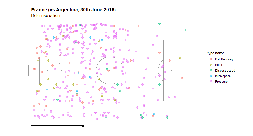
```{r}
d2 <- statsbomb %>%
filter(type.name %in% c("Pressure", "Interception", "Block", "Dispossessed", "Ball Recovery") & team.name == "France")
soccerPitch(arrow = "r",
title = "France (vs Argentina, 30th June 2016)",
subtitle = "Defensive actions") +
geom_point(data = d2, aes(x = location.x, y = location.y, col = type.name), size = 3, alpha = 0.5)
```
Start and end locations of passes:

```{r}
d3 <- statsbomb %>%
filter(type.name == "Pass" & team.name == "France") %>%
mutate(pass.outcome = as.factor(if_else(is.na(pass.outcome.name), 1, 0)))
soccerPitch(arrow = "r",
title = "France (vs Argentina, 30th June 2016)",
subtitle = "Pass map") +
geom_segment(data = d3, aes(x = location.x, xend = pass.end_location.x, y = location.y, yend = pass.end_location.y, col = pass.outcome), alpha = 0.75) +
geom_point(data = d3, aes(x = location.x, y = location.y, col = pass.outcome), alpha = 0.5) +
guides(colour = FALSE)
```
#### Player paths
Path of a single player:

```{r}
subset(tromso, id == 8)[1:1800,] %>%
soccerPath(col = "red", grass = TRUE, arrow = "r",
title = "Tromsø IL (vs. Strømsgodset, 3rd Nov 2013)",
subtitle = "Player #8 path (1' - 3')")
```
Path of multiple players:
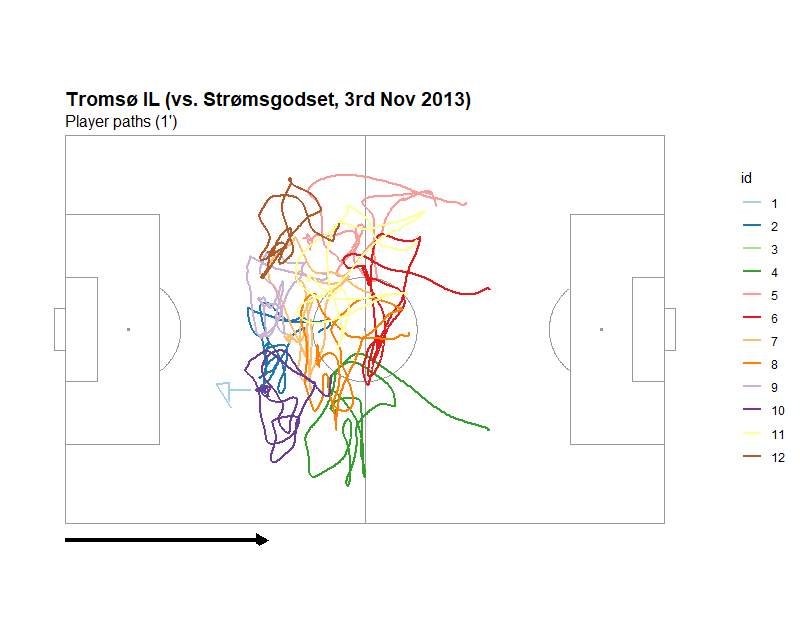
```{r}
tromso %>%
dplyr::group_by(id) %>%
dplyr::slice(1:1200) %>%
soccerPath(id = "id", arrow = "r",
title = "Tromsø IL (vs. Strømsgodset, 3rd Nov 2013)",
subtitle = "Player paths (1')")
```
---