Ecosyste.ms: Awesome
An open API service indexing awesome lists of open source software.
https://github.com/mschauer/Kalman.jl
Flexible filtering and smoothing in Julia
https://github.com/mschauer/Kalman.jl
filter kalman-filter kalman-smoother tracking
Last synced: about 2 months ago
JSON representation
Flexible filtering and smoothing in Julia
- Host: GitHub
- URL: https://github.com/mschauer/Kalman.jl
- Owner: mschauer
- License: other
- Created: 2018-02-01T09:15:17.000Z (over 6 years ago)
- Default Branch: master
- Last Pushed: 2023-04-19T19:51:12.000Z (about 1 year ago)
- Last Synced: 2024-05-10T16:08:08.899Z (about 2 months ago)
- Topics: filter, kalman-filter, kalman-smoother, tracking
- Language: Julia
- Homepage:
- Size: 692 KB
- Stars: 73
- Watchers: 5
- Forks: 10
- Open Issues: 6
-
Metadata Files:
- Readme: README.md
- License: LICENSE.md
Lists
- awesome-sciml - mschauer/Kalman.jl: Flexible filtering and smoothing in Julia
README
[](https://travis-ci.org/mschauer/Kalman.jl)
[](https://mschauer.github.io/Kalman.jl/latest/)
# Kalman
Flexible filtering and smoothing in Julia. `Kalman` uses [`DynamicIterators`](https://github.com/mschauer/DynamicIterators.jl) (an iterator protocol for dynamic data dependent and controlled processes) and
[`GaussianDistributions`](https://github.com/mschauer/GaussianDistributions.jl) (Gaussian distributions as abstraction for the uncertain state)
to implement flexible online Kalman filtering.
The package provides tools to filter and smooth and conditionally sample the state space system
x[k] = Φx[k−1] + b + w[k], w[k] ∼ N(0, Q)
y[k] = Hx[k] + v[k], v[k] ∼ N(0, R)
## How to use
One way, and maybe *the* way, to use this package is to use `Gaussian` from `GaussianDistributions.jl` as representation of mean and uncertainty of a filter and call `Kalman.correct` to implement the correction step in a Kalman filter:
```julia
using Kalman, GaussianDistributions, LinearAlgebra
using GaussianDistributions: ⊕ # independent sum of Gaussian r.v.
using Statistics
# prior for time 0
x0 = [-1., 1.]
P0 = Matrix(1.0I, 2, 2)
# dynamics
Φ = [0.8 0.2; -0.1 0.8]
b = zeros(2)
Q = [0.2 0.0; 0.0 0.5]
# observation
H = [1.0 0.0]
R = Matrix(0.3I, 1, 1)
# (mock) data
ys = [[-1.77], [-0.78], [-1.28], [-1.06], [-3.65], [-2.47], [-0.06], [-0.91], [-0.80], [1.48]]
# filter (assuming first observation at time 1)
N = length(ys)
p = Gaussian(x0, P0)
ps = [p] # vector of filtered Gaussians
for i in 1:N
global p
# predict
p = Φ*p ⊕ Gaussian(zero(x0), Q) #same as Gaussian(Φ*p.μ, Φ*p.Σ*Φ' + Q)
# correct
p, yres, _ = Kalman.correct(Kalman.JosephForm(), p, (Gaussian(ys[i], R), H))
push!(ps, p) # save filtered density
end
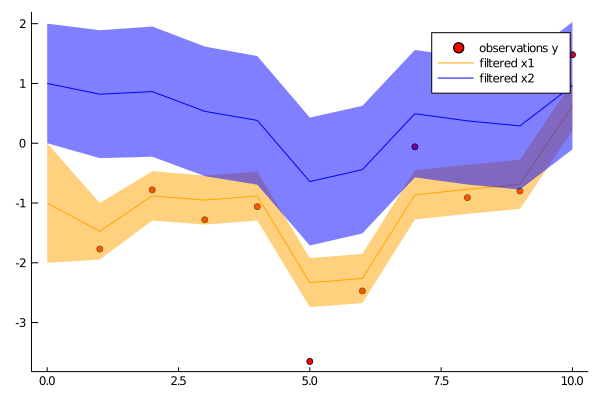
using Plots
p1 = scatter(1:N, first.(ys), color="red", label="observations y")
plot!(p1, 0:N, [mean(p)[1] for p in ps], color="orange", label="filtered x1", grid=false, ribbon=[sqrt(cov(p)[1,1]) for p in ps], fillalpha=.5)
plot!(p1, 0:N, [mean(p)[2] for p in ps], color="blue", label="filtered x2", grid=false, ribbon=[sqrt(cov(p)[2,2]) for p in ps], fillalpha=.5)
savefig(p1, "filter.png")
```
A very similar example of tracking a 2D trajectory can be found [here](example/trajectory_tracking/kalman.jl).
## Interface
The same might be achieved using interface functions
```julia
using DynamicIterators, GaussianDistributions, Kalman, LinearAlgebra
# Define linear evolution
Φ = [0.8 0.5; -0.1 0.8]
b = zeros(2)
Q = [0.2 0.0; 0.0 1.0]
E = LinearEvolution(Φ, Gaussian(b, Q))
# Define observation scheme
H = [1.0 0.0]
R = Matrix(1.0I, 1, 1)
O = LinearObservation(E, H, R)
# Prior
x0 = [1., 0.]
P0 = Matrix(1.0I, 2, 2)
# Observations (mock)
Y = [1 => [1.14326], 2 => [-0.271804], 3 => [-0.00512675]]
# Filter
Xf, ll = kalmanfilter(O, 0 => Gaussian(x0, P0), Y)
@show Xf
```
## Implementation
As said, filtering is implemented via the DynamicIterator protocol. It is worthwhile to look at
a possible the implementation of `kalmanfilter` to see how filtering can be integrated into online algorithms (run in a local scope to avoid `UndefVarError: ystate not defined`.)
```julia
# `Y` is the data iterator, iterating over pairs of `t => v` of time `t` and observation `v`
# `O` is the dynamical filter iterator, iterating over pairs `t => u` where
# u::Tuple{<:Gaussian,<:Gaussian,Float64}
# is the tuple of filtered state, the predicted state and the log likelihood
# Initialise data iterator
ϕ = iterate(Y)
ϕ === nothing && error("no observations")
(t, v), ystate = ϕ
# Initialise dynamical filter with first data point `t => v`
# and the `prior::Pair{Int,<:Gaussian}`, a pair of initial time and initial state
prior = 0 => Gaussian(x0, P0)
ϕ = dyniterate(O, Start(Kalman.Filter(prior, 0.0)), t => v)
ϕ === nothing && error("no observations")
(t, u), state = ϕ
X = [t => u[1]]
while true
# Advance data iterator
ϕ = iterate(Y, ystate)
ϕ === nothing && break
(t, v), ystate = ϕ
# Advance filter with new data `t => v`
ϕ = dyniterate(O, state, t => v)
ϕ === nothing && break
(t, u), state = ϕ
# Do something with the result `t => u` (here: saving it)
push!(X, t => u[1]) # save filtered state
end
ll = u[3] # likelihood
@show X, ll
```