https://github.com/SebKrantz/dfms
Dynamic Factor Models for R
https://github.com/SebKrantz/dfms
dynamic-factor-models rstats time-series
Last synced: 12 months ago
JSON representation
Dynamic Factor Models for R
- Host: GitHub
- URL: https://github.com/SebKrantz/dfms
- Owner: SebKrantz
- License: gpl-3.0
- Created: 2021-08-25T09:04:15.000Z (almost 5 years ago)
- Default Branch: main
- Last Pushed: 2025-06-17T00:28:53.000Z (about 1 year ago)
- Last Synced: 2025-06-17T01:28:13.373Z (about 1 year ago)
- Topics: dynamic-factor-models, rstats, time-series
- Language: R
- Homepage: https://sebkrantz.github.io/dfms/
- Size: 31.2 MB
- Stars: 37
- Watchers: 2
- Forks: 10
- Open Issues: 0
-
Metadata Files:
- Readme: README.md
- Changelog: NEWS.md
- Contributing: .github/CONTRIBUTING.md
- License: LICENSE
- Codemeta: codemeta.json
Awesome Lists containing this project
- jimsghstars - SebKrantz/dfms - Dynamic Factor Models for R (R)
README
# **dfms**: Dynamic Factor Models for R
[](https://github.com/ropensci/software-review/issues/556)
[](https://github.com/SebKrantz/dfms/actions)
[](https://sebkrantz.r-universe.dev)
[](https://cran.r-project.org/package=dfms)
[](https://cran.r-project.org/web/checks/check_results_dfms.html)


[](https://app.codecov.io/gh/SebKrantz/dfms?branch=main)
[](https://cran.r-project.org/)
[](https://CRAN.R-project.org/package=dfms)
*dfms* provides efficient estimation of Dynamic Factor Models via the EM Algorithm. Factors are assumed to follow a stationary VAR
process of order `p`. Estimation can be done in 3 different ways following:
- Doz, C., Giannone, D., & Reichlin, L. (2011). A two-step estimator for large approximate dynamic factor models based on Kalman filtering. *Journal of Econometrics, 164*(1), 188-205.
- Doz, C., Giannone, D., & Reichlin, L. (2012). A quasi-maximum likelihood approach for large, approximate dynamic factor models. *Review of Economics and Statistics, 94*(4), 1014-1024.
- Banbura, M., & Modugno, M. (2014). Maximum likelihood estimation of factor models on datasets with arbitrary pattern of missing data. *Journal of Applied Econometrics, 29*(1), 133-160.
The default is `em.method = "auto"`, which chooses `"BM"` following Banbura & Modugno (2014) with missing data or mixed frequency, and `"DGR"` following Doz, Giannone & Reichlin (2012) otherwise. Using `em.method = "none"` generates Two-Step estimates following Doz, Giannone & Reichlin (2011). This is extremely efficient on bigger datasets. PCA and Two-Step estimates are also reported in EM-estimation. All methods support missing data, but `em.method = "DGR"` does not model them in EM iterations.
The package is currently stable, but functionality may expand in the future. In particular, mixed-frequency estimation with autoregressive errors is planned for the near future, and generation of the 'news' may be added in the further future.
### Comparison with Other R Packages
*dfms* is intended to provide a simple, numerically robust, and computationally efficient baseline implementation of (linear Gaussian) Dynamic Factor Models for R, allowing straightforward application to various contexts such as time series dimensionality reduction and forecasting. The implementation is based on efficient C++ code, making *dfms* orders of magnitude faster than packages that can be used to fit dynamic factor models such as [*MARSS*](), or [*nowcasting*]() and [*nowcastDFM*]() geared to mixed-frequency nowcasting applications - supporting blocking of variables into different groups for which factors are to be estimated and evaluation of news content. For large-scale nowcasting models the [`DynamicFactorMQ`](https://www.statsmodels.org/dev/generated/statsmodels.tsa.statespace.dynamic_factor_mq.DynamicFactorMQ.html) class in the `statsmodels` Python library is probably the most robust implementation - see the [example](http://www.chadfulton.com/topics/statespace_large_dynamic_factor_models.html) by Chad Fulton.
The *dfms* package is not intended to fit more general forms of the state space model like [*MARSS*]().
### Installation
```r
# CRAN
install.packages("dfms")
# Development Version
install.packages('dfms', repos = c('https://sebkrantz.r-universe.dev', 'https://cloud.r-project.org'))
```
### Usage Example
```r
library(dfms)
# Fit DFM with 6 factors and 3 lags in the transition equation
mod <- DFM(diff(BM14_M), r = 6, p = 3)
```
```
## Converged after 32 iterations.
```
```r
# 'dfm' methods
summary(mod)
```
```
## Dynamic Factor Model: n = 92, T = 356, r = 6, p = 3, %NA = 25.8366
##
## Call: DFM(X = diff(BM14_M), r = 6, p = 3)
##
## Summary Statistics of Factors [F]
## N Mean Median SD Min Max
## f1 356 -0.1189 0.4409 4.0228 -22.9164 7.8513
## f2 356 -0.4615 -0.3476 2.9201 -9.0973 10.7003
## f3 356 -0.0173 0.0377 2.2719 -8.5067 7.3009
## f4 356 -0.007 -0.1338 1.9378 -9.5052 9.3673
## f5 356 0.237 0.1091 2.0857 -8.7252 9.6715
## f6 356 -0.8361 -0.304 3.1406 -11.6611 15.4897
##
## Factor Transition Matrix [A]
## L1.f1 L1.f2 L1.f3 L1.f4 L1.f5 L1.f6 L2.f1 L2.f2 L2.f3
## f1 0.53029 -0.53009 0.367302 0.04607 -0.06351 0.10310 0.02457 0.11673 -0.12638
## f2 -0.28380 0.07421 -0.032292 0.29741 -0.10094 0.21989 0.09958 -0.09149 0.06708
## f3 0.17607 0.12979 0.378798 -0.06662 -0.12236 0.06685 -0.08068 0.09101 -0.22232
## f4 0.02711 0.08936 0.004643 0.37159 0.12100 -0.02763 0.01234 -0.05147 0.02195
## f5 -0.26227 -0.03469 -0.046294 0.12712 0.26847 0.03141 0.06400 0.01971 0.04806
## f6 0.08251 0.17619 -0.013374 -0.08731 -0.03875 0.27812 -0.01662 0.04877 0.02279
## L2.f4 L2.f5 L2.f6 L3.f1 L3.f2 L3.f3 L3.f4 L3.f5 L3.f6
## f1 0.23135 0.117184 0.21941 0.18478 0.02259 -0.03719 -0.07236 -0.03026 -0.12606
## f2 -0.09768 -0.043057 0.08489 0.21107 0.16261 0.03057 0.04835 0.12249 0.13357
## f3 0.09799 -0.060666 -0.18028 -0.02773 0.01798 0.10143 -0.12420 0.04207 -0.07011
## f4 0.01266 0.050912 0.05144 -0.05601 0.04665 0.05710 -0.11412 -0.05680 -0.01609
## f5 -0.03965 -0.009952 -0.18471 0.08332 -0.04640 -0.02047 0.02458 0.16397 0.07820
## f6 0.01163 -0.100859 0.07152 0.00792 0.06071 0.11381 0.02520 -0.17897 0.30328
##
## Factor Covariance Matrix [cov(F)]
## f1 f2 f3 f4 f5 f6
## f1 16.1832 -0.4329 0.2483 -0.8224* -1.7708* 0.7702
## f2 -0.4329 8.5272 0.0051 0.2954 -0.2114 4.2080*
## f3 0.2483 0.0051 5.1614 -0.1851 -0.3979 0.2979
## f4 -0.8224* 0.2954 -0.1851 3.7550 0.4344* 0.2211
## f5 -1.7708* -0.2114 -0.3979 0.4344* 4.3503 -1.9785*
## f6 0.7702 4.2080* 0.2979 0.2211 -1.9785* 9.8634
##
## Factor Transition Error Covariance Matrix [Q]
## u1 u2 u3 u4 u5 u6
## u1 7.2142 0.1151 -0.8208 -0.4379 0.4110 -0.1206
## u2 0.1151 4.8724 0.1076 -0.1438 0.1418 0.1759
## u3 -0.8208 0.1076 4.0584 -0.0788 0.0163 0.0038
## u4 -0.4379 -0.1438 -0.0788 3.0003 0.2562 0.0243
## u5 0.4110 0.1418 0.0163 0.2562 2.8410 -0.1031
## u6 -0.1206 0.1759 0.0038 0.0243 -0.1031 2.9284
##
## Summary of Residual AR(1) Serial Correlations
## N Mean Median SD Min Max
## 92 -0.0644 -0.1024 0.2702 -0.5113 0.6674
##
## Summary of Individual R-Squared's
## N Mean Median SD Min Max
## 92 0.4556 0.4069 0.3041 0.0112 0.9989
```
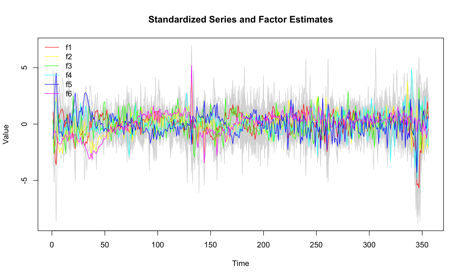
```r
plot(mod)
```
```r
as.data.frame(mod) |> head()
```
```
## Method Factor Time Value
## 1 PCA f1 1 0.8445713
## 2 PCA f1 2 0.5259228
## 3 PCA f1 3 -1.2107116
## 4 PCA f1 4 -1.5399532
## 5 PCA f1 5 -0.4631786
## 6 PCA f1 6 0.2399304
```
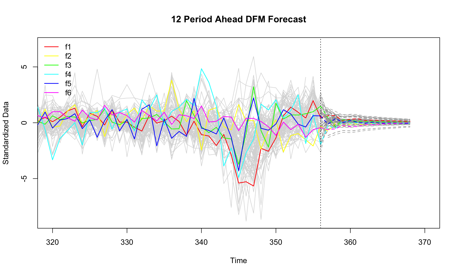
```r
# Forecasting 12 periods ahead
fc <- predict(mod, h = 12)
# 'dfm_forecast' methods
plot(fc, xlim = c(320, 370))
```
```r
as.data.frame(fc) |> head()
```
```
## Variable Time Forecast Value
## 1 f1 1 FALSE 4.179331
## 2 f1 2 FALSE -1.368577
## 3 f1 3 FALSE -12.845157
## 4 f1 4 FALSE -14.562265
## 5 f1 5 FALSE -7.791254
## 6 f1 6 FALSE -1.254970
```