https://github.com/analysiscenter/pydens
PyDEns is a framework for solving Ordinary and Partial Differential Equations (ODEs & PDEs) using neural networks
https://github.com/analysiscenter/pydens
deep-learning differential-equations neural-networks numerical-methods ode ode-solver partial-differential-equations pde-solver solving-pdes
Last synced: 7 months ago
JSON representation
PyDEns is a framework for solving Ordinary and Partial Differential Equations (ODEs & PDEs) using neural networks
- Host: GitHub
- URL: https://github.com/analysiscenter/pydens
- Owner: analysiscenter
- License: apache-2.0
- Created: 2019-07-16T13:20:34.000Z (about 7 years ago)
- Default Branch: master
- Last Pushed: 2024-02-09T09:55:29.000Z (over 2 years ago)
- Last Synced: 2025-11-14T07:22:21.391Z (8 months ago)
- Topics: deep-learning, differential-equations, neural-networks, numerical-methods, ode, ode-solver, partial-differential-equations, pde-solver, solving-pdes
- Language: Jupyter Notebook
- Homepage:
- Size: 23.8 MB
- Stars: 312
- Watchers: 14
- Forks: 67
- Open Issues: 13
-
Metadata Files:
- Readme: README.md
- License: LICENSE
Awesome Lists containing this project
README
[](https://www.apache.org/licenses/LICENSE-2.0)
[](https://python.org)
[](https://pytorch.org)
# PyDEns
**PyDEns** is a framework for solving Ordinary and Partial Differential Equations (ODEs & PDEs) using neural networks. With **PyDEns** one can solve
- PDEs & ODEs from a large family including [heat-equation](https://en.wikipedia.org/wiki/Heat_equation), [poisson equation](https://en.wikipedia.org/wiki/Poisson%27s_equation) and [wave-equation](https://en.wikipedia.org/wiki/Wave_equation)
- parametric families of PDEs
- PDEs with trainable coefficients.
This page outlines main capabilities of **PyDEns**. To get an in-depth understanding we suggest you to also read [the tutorial](https://github.com/analysiscenter/pydens/blob/master/tutorials/1.%20Solving%20PDEs.ipynb).
## Getting started with **PyDEns**: solving common PDEs
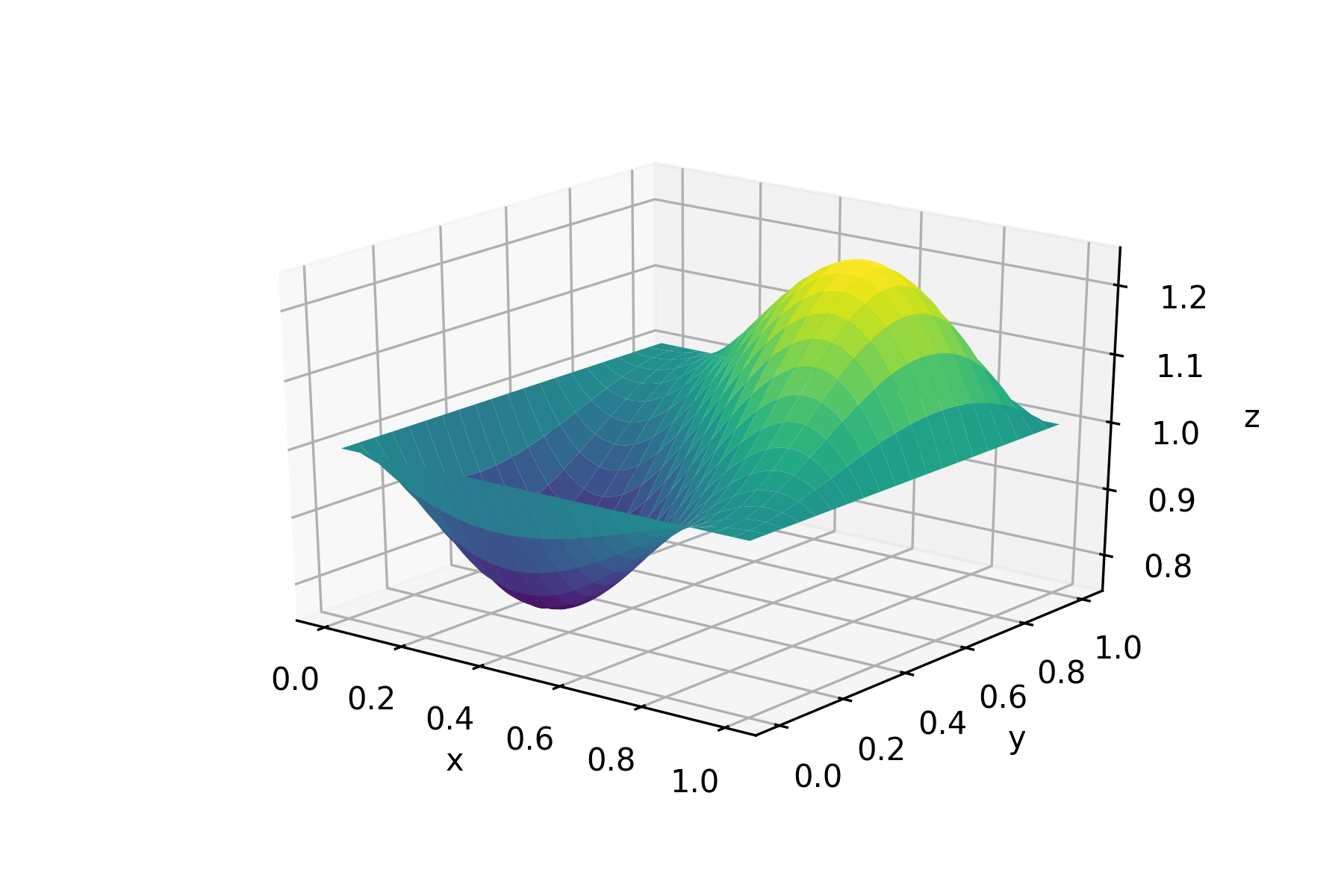
Let's solve poisson equation

using simple feed-forward neural network. Let's start by importing `Solver`-class along with other needed libraries:
```python
from pydens import Solver, NumpySampler
import numpy as np
import torch
```
You can now set up a **PyDEns**-model for solving the task at hand. For this you need to supply the equation into a `Solver`-instance. Note the use of differentiation token `D`:
```python
# Define the equation as a callable.
def pde(f, x, y):
return D(D(f, x), x) + D(D(f, y), y) - 5 * torch.sin(np.pi * (x + y))
# Supply the equation, initial condition, the number of variables (`ndims`)
# and the configration of neural network in Solver-instance.
solver = Solver(equation=pde, ndims=2, boundary_condition=1,
layout='fa fa fa f', activation='Tanh', units=[10, 12, 15, 1])
```
Note that we defined the architecture of the neural network by supplying `layout`, `activation` and `units` parameters. Here `layout` configures the sequence of layers: `fa fa fa f` stands for `f`ully connected architecture with four layers and three `a`ctivations. In its turn, `units` and `activation` cotrol the number of units in dense layers and activation-function. When defining neural network this way use [`ConvBlock`](https://analysiscenter.github.io/batchflow/api/batchflow.models.torch.layers.html?highlight=baseconvblock#batchflow.models.torch.layers.BaseConvBlock) from [`BatchFlow`](https://github.com/analysiscenter/batchflow).
It's time to run the optimization procedure
```python
solver.fit(batch_size=100, niters=1500)
```
in a fraction of second we've got a mesh-free approximation of the solution on **[0, 1]X[0, 1]**-square:
## Going deeper into **PyDEns**-capabilities
**PyDEns** allows to do much more than just solve common PDEs: it also deals with (i) parametric families of PDEs and (ii) PDEs with trainable coefficients.
### Solving parametric families of PDEs
Consider a *family* of ordinary differential equations

Clearly, the solution is a **sin** wave with a phase parametrized by ϵ:

Solving this problem is just as easy as solving common PDEs. You only need to introduce parameter `e` in the equation and supply the number of parameters (`nparams`) into a `Solver`-instance:
```python
def odeparam(f, x, e):
return D(f, x) - e * np.pi * torch.cos(e * np.pi * x)
# One for argument, one for parameter
s = NumpySampler('uniform') & NumpySampler('uniform', low=1, high=5)
solver = Solver(equation=odeparam, ndims=1, nparams=1, initial_condition=1)
solver.fit(batch_size=1000, sampler=s, niters=5000, lr=0.01)
# solving the whole family takes no more than a couple of seconds!
```
Check out the result:
### Solving PDEs with trainable coefficients
With **PyDEns** things can get even more interesting! Assume that the *initial state of the system is unknown and yet to be determined*:

Of course, without additional information, [the problem is undefined](https://en.wikipedia.org/wiki/Initial_value_problem). To make things better, let's fix the state of the system at some other point:

Setting this problem requires a [slightly more complex configuring](https://github.com/analysiscenter/pydens/blob/master/tutorials/PDE_solving.ipynb). Note the use of `V`-token, that stands for trainable variable, in the initial condition of the problem. Also pay attention to the additional constraint supplied into the `Solver` instance. This constraint binds the final solution to zero at `t=0.5`:
```python
def odevar(u, t):
return D(u, t) - 2 * np.pi * torch.cos(2 * np.pi * t)
def initial(*args):
return V('init', data=torch.Tensor([3.0]))
solver = Solver(odevar, ndims=1, initial_condition=initial,
constraints=lambda u, t: u(torch.tensor([0.5])))
```
When tackling this problem, `pydens` will not only solve the equation, but also adjust the variable (initial condition) to satisfy the additional constraint.
Hence, model-fitting comes in two parts now: (i) solving the equation and (ii) adjusting initial condition to satisfy the additional constraint. Inbetween
the steps we need to freeze layers of the network to adjust only the adjustable variable:
```python
solver.fit(batch_size=150, niters=100, lr=0.05)
solver.model.freeze_layers(['fc1', 'fc2', 'fc3'], ['log_scale'])
solver.fit(batch_size=150, niters=100, lr=0.05)
```
Check out the results:
## Installation
First of all, you have to manually install [pytorch](https://pytorch.org/get-started/locally/),
as you might need a certain version or a specific build for CPU / GPU.
### Stable python package
With modern [pipenv](https://docs.pipenv.org/)
```
pipenv install pydens
```
With old-fashioned [pip](https://pip.pypa.io/en/stable/)
```
pip3 install pydens
```
### Development version
```
pipenv install git+https://github.com/analysiscenter/pydens.git
```
```
pip3 install git+https://github.com/analysiscenter/pydens.git
```
### Installation as a project repository:
Do not forget to use the flag ``--recursive`` to make sure that ``BatchFlow`` submodule is also cloned.
```
git clone --recursive https://github.com/analysiscenter/pydens.git
```
In this case you need to manually install the dependencies.
## Citing PyDEns
Please cite **PyDEns** if it helps your research.
```
Roman Khudorozhkov, Sergey Tsimfer, Alexander Koryagin. PyDEns framework for solving differential equations with deep learning. 2019.
```
```
@misc{pydens_2019,
author = {Khudorozhkov R. and Tsimfer S. and Koryagin. A.},
title = {PyDEns framework for solving differential equations with deep learning},
year = 2019
}
```