https://github.com/chenqianhe/lenet5

Last synced: 3 months ago
JSON representation

Host: GitHub
URL: https://github.com/chenqianhe/lenet5
Owner: chenqianhe
Created: 2020-06-16T02:03:14.000Z (almost 5 years ago)
Default Branch: master
Last Pushed: 2020-06-16T02:06:06.000Z (almost 5 years ago)
Last Synced: 2025-01-19T18:17:59.294Z (5 months ago)
Language: Python
Size: 8.79 KB
Stars: 0
Watchers: 1
Forks: 0
Open Issues: 0
Metadata Files:
- Readme: README.md

Awesome Lists containing this project

README

# Paddle实现LeNet-5

## 一、LeNet-5介绍

手写字体识别模型LeNet5诞生于1994年，是最早的卷积神经网络之一。LeNet5通过巧妙的设计，利用卷积、参数共享、池化等操作提取特征，避免了大量的计算成本，最后再使用全连接神经网络进行分类识别，这个网络也是最近大量神经网络架构的起点。

LeNet5的网络结构示意图如下所示：
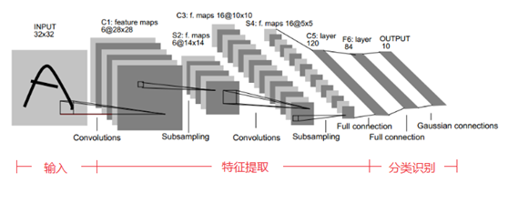
![这里写图片描述](https://static.oschina.net/uploads/space/2018/0311/012923_Ficx_876354.png)
LeNet5由7层CNN（不包含输入层）组成，上图中输入的原始图像大小是32×32像素，卷积层用Ci表示，子采样层（pooling，池化）用Si表示，全连接层用Fi表示。下面逐层介绍其作用和示意图上方的数字含义。
**1、C1层（卷积层）：6@28×28**
该层使用了6个卷积核，每个卷积核的大小为5×5，这样就得到了6个feature map（特征图）。
**（1）特征图大小**
每个卷积核（5×5）与原始的输入图像（32×32）进行卷积，这样得到的feature map（特征图）大小为（32-5+1）×（32-5+1）= 28×28

卷积核与输入图像按卷积核大小逐个区域进行匹配计算，匹配后原始输入图像的尺寸将变小，因为边缘部分卷积核无法越出界，只能匹配一次，匹配计算后的尺寸变为Cr×Cc=（Ir-Kr+1）×（Ic-Kc+1），其中Cr、Cc，Ir、Ic，Kr、Kc分别表示卷积后结果图像、输入图像、卷积核的行列大小。
**（2）参数个数**
由于参数（权值）共享的原因，对于同个卷积核每个神经元均使用相同的参数，因此，参数个数为（5×5+1）×6= 156，其中5×5为卷积核参数，1为偏置参数
**（3）连接数**
卷积后的图像大小为28×28，因此每个特征图有28×28个神经元，每个卷积核参数为（5×5+1）×6，因此，该层的连接数为（5×5+1）×6×28×28=122304
**2、S2层（下采样层，也称池化层）：6@14×14**
**（1）特征图大小**
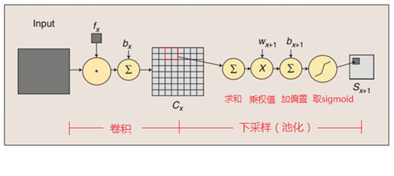
这一层主要是做池化或者特征映射（特征降维），池化单元为2×2，因此，6个特征图的大小经池化后即变为14×14。回顾本文刚开始讲到的池化操作，池化单元之间没有重叠，在池化区域内进行聚合统计后得到新的特征值，因此经2×2池化后，每两行两列重新算出一个特征值出来，相当于图像大小减半，因此卷积后的28×28图像经2×2池化后就变为14×14。
这一层的计算过程是：2×2 单元里的值相加，然后再乘以训练参数w，再加上一个偏置参数b（每一个特征图共享相同的w和b)，然后取sigmoid值（S函数：0-1区间），作为对应的该单元的值。卷积操作与池化的示意图如下：
![这里写图片描述](https://static.oschina.net/uploads/space/2018/0311/012957_l7Oh_876354.png)
**（2）参数个数**
S2层由于每个特征图都共享相同的w和b这两个参数，因此需要2×6=12个参数
**（3）连接数**
下采样之后的图像大小为14×14，因此S2层的每个特征图有14×14个神经元，每个池化单元连接数为2×2+1（1为偏置量），因此，该层的连接数为（2×2+1）×14×14×6 = 5880
**3、C3层（卷积层）：16@10×10**
C3层有16个卷积核，卷积模板大小为5×5。
**（1）特征图大小**
与C1层的分析类似，C3层的特征图大小为（14-5+1）×（14-5+1）= 10×10
**（2）参数个数**
需要注意的是，C3与S2并不是全连接而是部分连接，有些是C3连接到S2三层、有些四层、甚至达到6层，通过这种方式提取更多特征，连接的规则如下表所示：
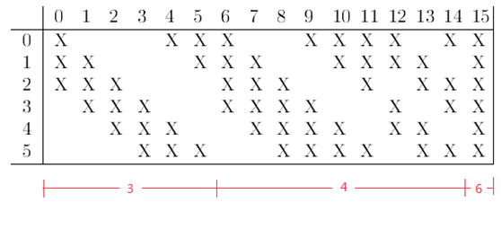
![这里写图片描述](https://static.oschina.net/uploads/space/2018/0311/013017_pIe9_876354.png)

例如第一列表示C3层的第0个特征图（feature map）只跟S2层的第0、1和2这三个feature maps相连接，计算过程为：用3个卷积模板分别与S2层的3个feature maps进行卷积，然后将卷积的结果相加求和，再加上一个偏置，再取sigmoid得出卷积后对应的feature map了。其它列也是类似（有些是3个卷积模板，有些是4个，有些是6个）。因此，C3层的参数数目为（5×5×3+1）×6 +（5×5×4+1）×9 +5×5×6+1 = 1516
**（3）连接数**
卷积后的特征图大小为10×10，参数数量为1516，因此连接数为1516×10×10= 151600
**4、S4（下采样层，也称池化层）：16@5×5**
**（1）特征图大小**
与S2的分析类似，池化单元大小为2×2，因此，该层与C3一样共有16个特征图，每个特征图的大小为5×5。
**（2）参数数量**
与S2的计算类似，所需要参数个数为16×2 = 32
**（3）连接数**
连接数为（2×2+1）×5×5×16 = 2000
**5、C5层（卷积层）：120**
**（1）特征图大小**
该层有120个卷积核，每个卷积核的大小仍为5×5，因此有120个特征图。由于S4层的大小为5×5，而该层的卷积核大小也是5×5，因此特征图大小为（5-5+1）×（5-5+1）= 1×1。这样该层就刚好变成了全连接，这只是巧合，如果原始输入的图像比较大，则该层就不是全连接了。
**（2）参数个数**
与前面的分析类似，本层的参数数目为120×（5×5×16+1） = 48120
**（3）连接数**
由于该层的特征图大小刚好为1×1，因此连接数为48120×1×1=48120
**6、F6层（全连接层）：84**
**（1）特征图大小**
F6层有84个单元，之所以选这个数字的原因是来自于输出层的设计，对应于一个7×12的比特图，如下图所示，-1表示白色，1表示黑色，这样每个符号的比特图的黑白色就对应于一个编码。
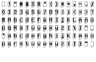
![这里写图片描述](https://static.oschina.net/uploads/space/2018/0311/013047_ApKN_876354.png)
该层有84个特征图，特征图大小与C5一样都是1×1，与C5层全连接。
**（2）参数个数**
由于是全连接，参数数量为（120+1）×84=10164。跟经典神经网络一样，F6层计算输入向量和权重向量之间的点积，再加上一个偏置，然后将其传递给sigmoid函数得出结果。
**（3）连接数**
由于是全连接，连接数与参数数量一样，也是10164。
**7、OUTPUT层（输出层）：10**
Output层也是全连接层，共有10个节点，分别代表数字0到9。如果第i个节点的值为0，则表示网络识别的结果是数字i。
**（1）特征图大小**
该层采用径向基函数（RBF）的网络连接方式，假设x是上一层的输入，y是RBF的输出，则RBF输出的计算方式是：
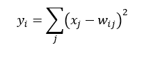
![这里写图片描述](https://static.oschina.net/uploads/space/2018/0311/013103_iVGG_876354.png)
上式中的Wij的值由i的比特图编码确定，i从0到9，j取值从0到7×12-1。RBF输出的值越接近于0，表示当前网络输入的识别结果与字符i越接近。
**（2）参数个数**
由于是全连接，参数个数为84×10=840
**（3）连接数**
由于是全连接，连接数与参数个数一样，也是840

## 二、Paddle实现

数据集为了简便我们仅采用MNIST作为案例，并且会对卷积和池化层的数量和大小略作更改，以获得更好的效果。

在Paddle中修改卷积和池化层都是非常方便的，只需要给出数量和大小即可，因此你也可以再去尝试一些其他的参数。

### 1.导入包

```python
import numpy as np
import paddle
import paddle.fluid as fluid
from PIL import Image
import matplotlib.pyplot as plt
import os
```

### 2.构造数据读取

Paddle提供了MNIST数据集和归一化

```python

BUF_SIZE = 512
BATCH_SIZE = 128

train_reader = paddle.batch(
paddle.reader.shuffle(paddle.dataset.mnist.train(),
buf_size = BUF_SIZE),
batch_size = BATCH_SIZE)

test_reader = paddle.batch(
paddle.reader.shuffle(paddle.dataset.mnist.test(),
buf_size = BUF_SIZE),
batch_size = BATCH_SIZE)

train_data = paddle.dataset.mnist.train()
sampledata = next(train_data())
print(sampledata)
```

```
(array([-1. , -1. , -1. , -1. , -1. ,
-1. , -1. , -1. , -1. , -1. ,
-1. , -1. , -1. , -1. , -1. ,
-1. , -1. , -1. , -1. , -1. ,
-1. , -1. , -1. , -1. , -1. ,
-1. , -1. , -1. , -1. , -1. ,
-1. , -1. , -1. , -1. , -1. ,
-1. , -1. , -1. , -1. , -1. ,
-1. , -1. , -1. , -1. , -1. ,
-1. , -1. , -1. , -1. , -1. ,
-1. , -1. , -1. , -1. , -1. ,
-1. , -1. , -1. , -1. , -1. ,
-1. , -1. , -1. , -1. , -1. ,
-1. , -1. , -1. , -1. , -1. ,
-1. , -1. , -1. , -1. , -1. ,
-1. , -1. , -1. , -1. , -1. ,
-1. , -1. , -1. , -1. , -1. ,
-1. , -1. , -1. , -1. , -1. ,
-1. , -1. , -1. , -1. , -1. ,
-1. , -1. , -1. , -1. , -1. ,
-1. , -1. , -1. , -1. , -1. ,
-1. , -1. , -1. , -1. , -1. ,
-1. , -1. , -1. , -1. , -1. ,
-1. , -1. , -1. , -1. , -1. ,
-1. , -1. , -1. , -1. , -1. ,
-1. , -1. , -1. , -1. , -1. ,
-1. , -1. , -1. , -1. , -1. ,
-1. , -1. , -1. , -1. , -1. ,
-1. , -1. , -1. , -1. , -1. ,
-1. , -1. , -1. , -1. , -1. ,
-1. , -1. , -0.9764706 , -0.85882354, -0.85882354,
-0.85882354, -0.01176471, 0.06666672, 0.37254906, -0.79607844,
0.30196083, 1. , 0.9372549 , -0.00392157, -1. ,
-1. , -1. , -1. , -1. , -1. ,
-1. , -1. , -1. , -1. , -1. ,
-1. , -0.7647059 , -0.7176471 , -0.26274508, 0.20784318,
0.33333337, 0.9843137 , 0.9843137 , 0.9843137 , 0.9843137 ,
0.9843137 , 0.7647059 , 0.34901965, 0.9843137 , 0.8980392 ,
0.5294118 , -0.4980392 , -1. , -1. , -1. ,
-1. , -1. , -1. , -1. , -1. ,
-1. , -1. , -1. , -0.6156863 , 0.8666667 ,
0.9843137 , 0.9843137 , 0.9843137 , 0.9843137 , 0.9843137 ,
0.9843137 , 0.9843137 , 0.9843137 , 0.96862745, -0.27058822,
-0.35686272, -0.35686272, -0.56078434, -0.69411767, -1. ,
-1. , -1. , -1. , -1. , -1. ,
-1. , -1. , -1. , -1. , -1. ,
-1. , -0.85882354, 0.7176471 , 0.9843137 , 0.9843137 ,
0.9843137 , 0.9843137 , 0.9843137 , 0.5529412 , 0.427451 ,
0.9372549 , 0.8901961 , -1. , -1. , -1. ,
-1. , -1. , -1. , -1. , -1. ,
-1. , -1. , -1. , -1. , -1. ,
-1. , -1. , -1. , -1. , -1. ,
-0.372549 , 0.22352946, -0.1607843 , 0.9843137 , 0.9843137 ,
0.60784316, -0.9137255 , -1. , -0.6627451 , 0.20784318,
-1. , -1. , -1. , -1. , -1. ,
-1. , -1. , -1. , -1. , -1. ,
-1. , -1. , -1. , -1. , -1. ,
-1. , -1. , -1. , -1. , -0.8901961 ,
-0.99215686, 0.20784318, 0.9843137 , -0.29411763, -1. ,
-1. , -1. , -1. , -1. , -1. ,
-1. , -1. , -1. , -1. , -1. ,
-1. , -1. , -1. , -1. , -1. ,
-1. , -1. , -1. , -1. , -1. ,
-1. , -1. , -1. , -1. , 0.09019613,
0.9843137 , 0.4901961 , -0.9843137 , -1. , -1. ,
-1. , -1. , -1. , -1. , -1. ,
-1. , -1. , -1. , -1. , -1. ,
-1. , -1. , -1. , -1. , -1. ,
-1. , -1. , -1. , -1. , -1. ,
-1. , -1. , -0.9137255 , 0.4901961 , 0.9843137 ,
-0.45098037, -1. , -1. , -1. , -1. ,
-1. , -1. , -1. , -1. , -1. ,
-1. , -1. , -1. , -1. , -1. ,
-1. , -1. , -1. , -1. , -1. ,
-1. , -1. , -1. , -1. , -1. ,
-1. , -0.7254902 , 0.8901961 , 0.7647059 , 0.254902 ,
-0.15294117, -0.99215686, -1. , -1. , -1. ,
-1. , -1. , -1. , -1. , -1. ,
-1. , -1. , -1. , -1. , -1. ,
-1. , -1. , -1. , -1. , -1. ,
-1. , -1. , -1. , -1. , -1. ,
-0.36470586, 0.88235295, 0.9843137 , 0.9843137 , -0.06666666,
-0.8039216 , -1. , -1. , -1. , -1. ,
-1. , -1. , -1. , -1. , -1. ,
-1. , -1. , -1. , -1. , -1. ,
-1. , -1. , -1. , -1. , -1. ,
-1. , -1. , -1. , -1. , -0.64705884,
0.45882356, 0.9843137 , 0.9843137 , 0.17647064, -0.7882353 ,
-1. , -1. , -1. , -1. , -1. ,
-1. , -1. , -1. , -1. , -1. ,
-1. , -1. , -1. , -1. , -1. ,
-1. , -1. , -1. , -1. , -1. ,
-1. , -1. , -1. , -0.8745098 , -0.27058822,
0.9764706 , 0.9843137 , 0.4666667 , -1. , -1. ,
-1. , -1. , -1. , -1. , -1. ,
-1. , -1. , -1. , -1. , -1. ,
-1. , -1. , -1. , -1. , -1. ,
-1. , -1. , -1. , -1. , -1. ,
-1. , -1. , -1. , 0.9529412 , 0.9843137 ,
0.9529412 , -0.4980392 , -1. , -1. , -1. ,
-1. , -1. , -1. , -1. , -1. ,
-1. , -1. , -1. , -1. , -1. ,
-1. , -1. , -1. , -1. , -1. ,
-1. , -1. , -1. , -0.6392157 , 0.0196079 ,
0.43529415, 0.9843137 , 0.9843137 , 0.62352943, -0.9843137 ,
-1. , -1. , -1. , -1. , -1. ,
-1. , -1. , -1. , -1. , -1. ,
-1. , -1. , -1. , -1. , -1. ,
-1. , -1. , -1. , -1. , -0.69411767,
0.16078436, 0.79607844, 0.9843137 , 0.9843137 , 0.9843137 ,
0.9607843 , 0.427451 , -1. , -1. , -1. ,
-1. , -1. , -1. , -1. , -1. ,
-1. , -1. , -1. , -1. , -1. ,
-1. , -1. , -1. , -1. , -1. ,
-0.8117647 , -0.10588235, 0.73333335, 0.9843137 , 0.9843137 ,
0.9843137 , 0.9843137 , 0.5764706 , -0.38823527, -1. ,
-1. , -1. , -1. , -1. , -1. ,
-1. , -1. , -1. , -1. , -1. ,
-1. , -1. , -1. , -1. , -1. ,
-1. , -0.81960785, -0.4823529 , 0.67058825, 0.9843137 ,
0.9843137 , 0.9843137 , 0.9843137 , 0.5529412 , -0.36470586,
-0.9843137 , -1. , -1. , -1. , -1. ,
-1. , -1. , -1. , -1. , -1. ,
-1. , -1. , -1. , -1. , -1. ,
-1. , -1. , -0.85882354, 0.3411765 , 0.7176471 ,
0.9843137 , 0.9843137 , 0.9843137 , 0.9843137 , 0.5294118 ,
-0.372549 , -0.92941177, -1. , -1. , -1. ,
-1. , -1. , -1. , -1. , -1. ,
-1. , -1. , -1. , -1. , -1. ,
-1. , -1. , -1. , -0.5686275 , 0.34901965,
0.77254903, 0.9843137 , 0.9843137 , 0.9843137 , 0.9843137 ,
0.9137255 , 0.04313731, -0.9137255 , -1. , -1. ,
-1. , -1. , -1. , -1. , -1. ,
-1. , -1. , -1. , -1. , -1. ,
-1. , -1. , -1. , -1. , -1. ,
-1. , 0.06666672, 0.9843137 , 0.9843137 , 0.9843137 ,
0.6627451 , 0.05882359, 0.03529418, -0.8745098 , -1. ,
-1. , -1. , -1. , -1. , -1. ,
-1. , -1. , -1. , -1. , -1. ,
-1. , -1. , -1. , -1. , -1. ,
-1. , -1. , -1. , -1. , -1. ,
-1. , -1. , -1. , -1. , -1. ,
-1. , -1. , -1. , -1. , -1. ,
-1. , -1. , -1. , -1. , -1. ,
-1. , -1. , -1. , -1. , -1. ,
-1. , -1. , -1. , -1. , -1. ,
-1. , -1. , -1. , -1. , -1. ,
-1. , -1. , -1. , -1. , -1. ,
-1. , -1. , -1. , -1. , -1. ,
-1. , -1. , -1. , -1. , -1. ,
-1. , -1. , -1. , -1. , -1. ,
-1. , -1. , -1. , -1. , -1. ,
-1. , -1. , -1. , -1. , -1. ,
-1. , -1. , -1. , -1. , -1. ,
-1. , -1. , -1. , -1. , -1. ,
-1. , -1. , -1. , -1. , -1. ,
-1. , -1. , -1. , -1. ], dtype=float32), 5)
```

### 3.定义网络结构

首先定义输入的二维图像，之后经过两个卷积池化层，再经过全连接层，最后使用Softmax作为激活函数的全连接层作为输出层。

第一个卷积池化使用20个5*5的滤波器，池大小为2，步长为2

第一个卷积池化使用50个5*5的滤波器，池大小为2，步长为2

```python
def convolutional_neural_network():

img = fluid.layers.data(name='img', shape=[1, 28, 28], dtype='float32')

conv_pool_1 = fluid.nets.simple_img_conv_pool(
input=img,
filter_size=5,
num_filters=20,
pool_size=2,
pool_stride=2,
act='relu'
)
conv_pool_1 = fluid.layers.batch_norm(conv_pool_1)

conv_pool_2 = fluid.nets.simple_img_conv_pool(
input=conv_pool_1,
filter_size=5,
num_filters=50,
pool_size=2,
pool_stride=2,
act='relu'
)
prediction = fluid.layers.fc(input=conv_pool_2, size=10, act='softmax')

return prediction
```

### 4.配置train_program

```python
def train_program():
label = fluid.layers.data(name='label', shape=[1], dtype='int64')
predict = convolutional_neural_network()

cost = fluid.layers.cross_entropy(input=predict, label=label)

avg_cost = fluid.layers.mean(cost)

acc = fluid.layers.accuracy(input=predict, label=label)

return predict, [avg_cost, acc]

```

### 5.配置优化器

```python

def optimizer_program():
return fluid.optimizer.Adam(learning_rate=1e-3)
```

### 6.事件处理配置

```python
def event_handler(pass_id, batch_id, cost):
print("Pass %d, Batch %d, Cost %f" % (pass_id, batch_id, cost))
```

```python

from paddle.utils.plot import Ploter

train_prompt = "Train cost"
test_prompt = "Test cost"
cost_ploter = Ploter(train_prompt, test_prompt)

def event_handler_plot(ploter_title, step, cost):
cost_ploter.append(ploter_title, step, cost)
cost_ploter.plot()
```

### 7.定义网络配置

```python
use_cuda = True
place = fluid.CUDAPlace(0) if use_cuda else fluid.CPUPlace

prediction, [avg_loss, acc] = train_program()

img = fluid.layers.data(name='img', shape=[1, 28, 28], dtype='float32')

label = fluid.layers.data(name='label', shape=[1], dtype='int64')

feeder = fluid.DataFeeder(feed_list=[img, label], place=place)

optimizer = optimizer_program()
opts = optimizer.minimize(avg_loss)
```

### 8.设置超参数

```python
PASS_NUM = 10
epoch = [epoch_id for epoch_id in range(PASS_NUM)]

save_dirname = "recognize_digits.inference.model"
```

### 9.设置模型预测方法

```python
def train_test(train_test_program, train_test_feed, train_test_reader):
acc_set = []

avg_loss_set = []

for test_data in train_test_reader():
acc_np, avg_loss_np = exe.run(
program=train_test_program,
feed=train_test_feed.feed(test_data),
fetch_list=[acc, avg_loss]
)
acc_set.append(float(acc_np))
avg_loss_set.append(float(avg_loss_np))

acc_val_mean = np.array(acc_set).mean()
avg_loss_val_mean = np.array(avg_loss_set).mean()

return avg_loss_val_mean, acc_val_mean
```

### 10.创建执行器

```python
exe = fluid.Executor(place)
exe.run(fluid.default_startup_program())
```

### 11.设置main_program和test_program

```python
main_program = fluid.default_main_program()
test_program = fluid.default_main_program().clone(for_test=True)
```

### 12.开始训练

```python
lists = []
step = 0
for epoch_id in epoch:
for step_id, data in enumerate(train_reader()):
metrics = exe.run(main_program,
feed=feeder.feed(data),
fetch_list=[avg_loss, acc])
if step % 100 == 0:
event_handler(step, epoch_id, metrics[0])

# event_handler_plot(train_prompt, step, metrics[0])

step += 1

print("finish")

avg_loss_val, acc_val = train_test(train_test_program=test_program,
train_test_reader=test_reader,
train_test_feed=feeder)

print("Test with Epoch %d, avg_cost: %s, acc: %s" % (epoch_id, avg_loss_val, acc_val))
# event_handler_plot(test_prompt, step, metrics[0])

lists.append((epoch_id, avg_loss_val, acc_val))

if save_dirname is not None:
fluid.io.save_inference_model(save_dirname,
["img"], [prediction], exe,
model_filename=None,
params_filename=None)
```

```
Pass 0, Batch 0, Cost 4.914942
Pass 100, Batch 0, Cost 0.289003
Pass 200, Batch 0, Cost 0.166288
Pass 300, Batch 0, Cost 0.044977
Pass 400, Batch 0, Cost 0.070677
finish
Test with Epoch 0, avg_cost: 0.07840685797501591, acc: 0.9733979430379747
Pass 500, Batch 1, Cost 0.057925
Pass 600, Batch 1, Cost 0.016752
Pass 700, Batch 1, Cost 0.069734
Pass 800, Batch 1, Cost 0.060028
Pass 900, Batch 1, Cost 0.072877
finish
Test with Epoch 1, avg_cost: 0.05281242278781779, acc: 0.9817049050632911
Pass 1000, Batch 2, Cost 0.088036
Pass 1100, Batch 2, Cost 0.119314
Pass 1200, Batch 2, Cost 0.008125
Pass 1300, Batch 2, Cost 0.024729
Pass 1400, Batch 2, Cost 0.005659
finish
Test with Epoch 2, avg_cost: 0.04380615004831984, acc: 0.985067246835443
Pass 1500, Batch 3, Cost 0.059868
Pass 1600, Batch 3, Cost 0.042946
Pass 1700, Batch 3, Cost 0.074827
Pass 1800, Batch 3, Cost 0.058897
finish
Test with Epoch 3, avg_cost: 0.04563218841618045, acc: 0.9840783227848101
Pass 1900, Batch 4, Cost 0.002829
Pass 2000, Batch 4, Cost 0.065684
Pass 2100, Batch 4, Cost 0.015218
Pass 2200, Batch 4, Cost 0.011254
Pass 2300, Batch 4, Cost 0.013128
finish
Test with Epoch 4, avg_cost: 0.055302140963410434, acc: 0.9821993670886076
Pass 2400, Batch 5, Cost 0.030149
Pass 2500, Batch 5, Cost 0.000964
Pass 2600, Batch 5, Cost 0.016074
Pass 2700, Batch 5, Cost 0.025854
Pass 2800, Batch 5, Cost 0.008434
finish
Test with Epoch 5, avg_cost: 0.0566819144060682, acc: 0.983682753164557
Pass 2900, Batch 6, Cost 0.010033
Pass 3000, Batch 6, Cost 0.002197
Pass 3100, Batch 6, Cost 0.022742
Pass 3200, Batch 6, Cost 0.023751
finish
Test with Epoch 6, avg_cost: 0.05313029858223649, acc: 0.9854628164556962
Pass 3300, Batch 7, Cost 0.002085
Pass 3400, Batch 7, Cost 0.013630
Pass 3500, Batch 7, Cost 0.006875
Pass 3600, Batch 7, Cost 0.004274
Pass 3700, Batch 7, Cost 0.000854
finish
Test with Epoch 7, avg_cost: 0.06596997759859019, acc: 0.9821004746835443
Pass 3800, Batch 8, Cost 0.001887
Pass 3900, Batch 8, Cost 0.003138
Pass 4000, Batch 8, Cost 0.016411
Pass 4100, Batch 8, Cost 0.000250
Pass 4200, Batch 8, Cost 0.058225
finish
Test with Epoch 8, avg_cost: 0.06523720332980598, acc: 0.9838805379746836
Pass 4300, Batch 9, Cost 0.001661
Pass 4400, Batch 9, Cost 0.006142
Pass 4500, Batch 9, Cost 0.000767
Pass 4600, Batch 9, Cost 0.005788
finish
Test with Epoch 9, avg_cost: 0.0692533968895883, acc: 0.9822982594936709
```

### 13.取得最好的模型

```python
best = sorted(lists, key=lambda list:float(list[1]))[0]
print('Best pass is %s, testing Avgcost is %s' % (best[0], best[1]))
print('The classification accuracy is %.2f%%' % (float(best[2])*100))
```

```
Best pass is 2, testing Avgcost is 0.04380615004831984
The classification accuracy is 98.51%
```

## 三、程序地址

Github: https://github.com/chenqianhe/LeNet5

AIstudio： https://aistudio.baidu.com/aistudio/projectdetail/551501

ecosyste.ms

Data

Tools

Indexes

Applications

Experiments

Awesome

https://github.com/chenqianhe/lenet5

Awesome Lists containing this project

README