https://github.com/christophmark/bayesianfridge
Sequential Monte Carlo sampler for PyMC2 models.
https://github.com/christophmark/bayesianfridge
inference inference-engine model-selection monte-carlo sequential-monte-carlo
Last synced: 11 months ago
JSON representation
Sequential Monte Carlo sampler for PyMC2 models.
- Host: GitHub
- URL: https://github.com/christophmark/bayesianfridge
- Owner: christophmark
- License: mit
- Created: 2018-04-04T11:04:43.000Z (about 8 years ago)
- Default Branch: master
- Last Pushed: 2018-04-04T11:20:16.000Z (about 8 years ago)
- Last Synced: 2024-11-19T09:37:03.502Z (over 1 year ago)
- Topics: inference, inference-engine, model-selection, monte-carlo, sequential-monte-carlo
- Language: Python
- Size: 54.7 KB
- Stars: 13
- Watchers: 3
- Forks: 3
- Open Issues: 0
-
Metadata Files:
- Readme: README.md
- License: LICENSE
Awesome Lists containing this project
README

[](https://opensource.org/licenses/MIT)
[](https://zenodo.org/badge/latestdoi/128050340)
This package implements Bayesian annealed sequential importance sampling (BASIS), a Sequential Monte Carlo sampling technique described by [Wu2017](https://doi.org/10.1115/1.4037450). In particular, it implements the special case with a maximum chain length of one (l_max = 1). Sequential Monte Carlo methods stand out against MCMC or HMC methods as they are able to estimate the model evidence (also called marginal likelihood) which can be used to objectively compare models of varying complexity. We combine the algorithm by [Wu2017](https://doi.org/10.1115/1.4037450) with an optional tuning method for the proposal scaling factor beta, as described by [Minson2013](https://doi.org/10.1093/gji/ggt180). The sample function can perform parameter inference and model selection on any valid [PyMC2](https://pymc-devs.github.io/pymc/)-model object.
## Installation
The easiest way to install the latest release version of *bayesianfridge* is via `pip`:
```
pip install bayesianfridge
```
Alternatively, a zipped version can be downloaded [here](https://github.com/christophmark/bayesianfridge/releases). The module is installed by calling `python setup.py install`.
## Development version
The latest development version of *bayesianfridge* can be installed from the master branch using pip (requires git):
```
pip install git+https://github.com/christophmark/bayesianfridge
```
Alternatively, use this [zipped version](https://github.com/christophmark/bayesianfridge/zipball/master) or clone the repository.
## Getting started
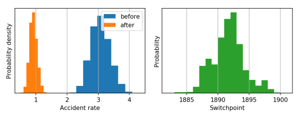
The following code provides a minimal example of an analysis carried out using *bayesloop*. The data here consists of the number of coal mining disasters in the UK per year from 1851 to 1962 (see this [article](https://academic.oup.com/biomet/article-pdf/66/1/191/600109/66-1-191.pdf) for further information). This example is also discussed in the official [PyMC2 documentation](https://pymc-devs.github.io/pymc/tutorial.html).
```
import numpy as np
import pymc
from bayesianfridge import sample
import matplotlib.pyplot as plt
data = np.array([5, 4, 1, 0, 4, 3, 4, 0, 6, 3, 3, 4, 0, 2, 6, 3, 3, 5, 4, 5, 3, 1, 4,
4, 1, 5, 5, 3, 4, 2, 5, 2, 2, 3, 4, 2, 1, 3, 2, 2, 1, 1, 1, 1, 3, 0,
0, 1, 0, 1, 1, 0, 0, 3, 1, 0, 3, 2, 2, 0, 1, 1, 1, 0, 1, 0, 1, 0, 0,
0, 2, 1, 0, 0, 0, 1, 1, 0, 2, 3, 3, 1, 1, 2, 1, 1, 1, 1, 2, 3, 3, 0,
0, 0, 1, 4, 0, 0, 0, 1, 0, 0, 0, 0, 0, 1, 0, 0, 1, 0])
# Probabilistic model
switchpoint = pymc.DiscreteUniform('switchpoint', lower=0, upper=110)
early_mean = pymc.Exponential('early_mean', beta=1.)
late_mean = pymc.Exponential('late_mean', beta=1.)
@pymc.deterministic
def rate(s=switchpoint, e=early_mean, l=late_mean):
out = np.empty(len(data))
out[:s] = e
out[s:] = l
return out
obs = pymc.Poisson('disasters', mu=rate, value=data, observed=True)
model = pymc.Model([switchpoint, early_mean, late_mean, obs])
# Inference
samples, marglike = sample(model, 10000)
# Plotting
m1 = samples['early_mean']
t = samples['switchpoint'] + 1852
m2 = samples['late_mean']
plt.figure()
plt.subplot2grid((1, 2), (0, 0))
plt.hist(m1, facecolor='C0', label='before')
plt.hist(m2, facecolor='C1', label='after')
plt.xlabel('Accident rate')
plt.ylabel('Probability density')
plt.yticks([])
plt.grid()
plt.legend()
plt.subplot2grid((1, 2), (0, 1))
plt.hist(t, bins=range(int(min(t)), int(max(t)) + 1, 1), facecolor='C2')
plt.xlabel('Switchpoint')
plt.ylabel('Probability')
plt.yticks([])
plt.grid()
```
## License
[The MIT License (MIT)](https://github.com/christophmark/bayesianfridge/blob/master/LICENSE)