https://github.com/corey-richardson/microbit-data-logger
In preparation for Work Experience Students coming in, I am using this project to familiarise myself with the BBC micro:bits which we will provide them with. I am also using it as a chance to expand on my data visualisation with Python experience.
https://github.com/corey-richardson/microbit-data-logger
data-visualization matplotlib microbit pandas pyplot signal-processing
Last synced: about 2 months ago
JSON representation
In preparation for Work Experience Students coming in, I am using this project to familiarise myself with the BBC micro:bits which we will provide them with. I am also using it as a chance to expand on my data visualisation with Python experience.
- Host: GitHub
- URL: https://github.com/corey-richardson/microbit-data-logger
- Owner: corey-richardson
- Created: 2023-06-07T11:53:01.000Z (about 3 years ago)
- Default Branch: main
- Last Pushed: 2023-07-04T07:25:57.000Z (almost 3 years ago)
- Last Synced: 2025-02-05T14:40:58.758Z (over 1 year ago)
- Topics: data-visualization, matplotlib, microbit, pandas, pyplot, signal-processing
- Language: Python
- Homepage:
- Size: 35.3 MB
- Stars: 0
- Watchers: 1
- Forks: 0
- Open Issues: 0
-
Metadata Files:
- Readme: README.md
Awesome Lists containing this project
README
# Data Logger Project
[](https://github.com/corey-richardson/microbit-data-logger/actions/workflows/check.yaml)
---
## Contents
- [aims](#aims)
- [concerns](#concerns)
- [relevant-practice-projects](#relevant-practice-projects)
- [microbit-xyz-planes-and-orientations](#microbit-xyz-planes-and-orientation)
- [flashing-to-microbit-using-web-based-text-editor](#flashing-to-microbit-using-web-based-text-editor)
Data Logging Visualisation via Serial Port
- [visualing-the-microbit-data-via-usb-cable](#visualing-the-microbit-data-via-usb-cable)
- [serial-port-writer-mainpy](#serial-port-writer-mainpy)
- [serial-port-reader-and-realtime-visualiser](#serial-port-reader-and-realtime-visualiser)
- [serial-port-reader-and-3d-realtime-visualiser](#serial-port-reader-and-3d-realtime-visualiser)
Data Logging Visualisation via CSV Files
- [visualing-the-microbit-with-csv-data](#visualing-the-microbit-with-csv-data)
- [process](#process)
- [csv-data-writer-mainpy](#csv-data-writer-mainpy)
- [csv-data-visualiser](#csv-data-visualiser)
- [csv-data-3d-visualiser](#csv-data-3d-visualiser)
Output GIFS
- [output](#output)
- [serial-port-connection](#serial-port-connection)
- [from-csv-data](#from-csv-data)
Final Project and Presentation - Archery Data Logger
- [final-project-and-presentation](#final-project-and-presentation)
- [project-selection](#project-selection)
- [why](#why)
- [plan](#plan)
- [what-went-well](#what-went-well)
- [lessons-learned](#lessons-learned)
- [testing-and-results](#testing-and-results)
- [potential-application](#potential-application)
---
## Aims
- Find the process of flashing software to the BBC micro:bit
- Use one of the micro:bit practice projects to familarise myself with the micro:bit capabilities and process; [data-logging-project](https://microbit.org/get-started/user-guide/data-logging/)
- Use Python scripts to output the data as graphs.
- This could be done as a realtime data logger or as plots taken from `.csv` data.
- Create a presentation on a "commercial product" using the micro:bit, writing about the following stages:
- Project Selection
- Why?
- What Went Well
- Lessons Learned
- Testing and Results
- Potential Application
> This could be used by the students as an example of what their presentations should consist of.
- All the while, thnk of how this could be tailored to students of varying experience levels and interests.
- MakeCode Blocks vs Python
- How could it be linked to their interests?
---
## Concerns
- [x] Is micro:bit storage non-volatile? *(Will the logs be erased when it is unplugged from power?)*
> Data is stored on your micro:bit even when the power is disconnected. It's easy to access - no software is needed. Plug your micro:bit in to a computer, look in the MICROBIT drive and double-click the MY_DATA file to open it in a web browser.
- [x] Does the micro:bit have enough storage space to record data for the time frames I'm hoping to record?
> Memory: 128 KB. Flash space: 512 KB.
- [x] Can I install Pip / PyPI Modules on a work laptop?
> :x: Pip / PyPI cannot be used to install Python packages on a work laptop. A different idea would be to supply the students with an executable version of the various plotting scripts. These `.exe` files could be created with [auto-py-to-exe](https://pypi.org/project/auto-py-to-exe/).
- I believe I have all dependencies other than `PySerial` installed, would a USB transfer from an external device be possible?
- [x] Need to verify if micro:bit will work on work laptop.
> :red_circle: Works with USB R/W permissions, not with Read Only Permissions. May have to use non-networked laptops OR the BBC micro:bit app.
- [ ] If the students are going to do data analysis via Excel, it will have to be installed for them onto a non-networked laptop. Same applies if they want to use Python or Matlab etc.
---
## Relevant Practice Projects
- [micro:bit Projects](https://microbit.org/projects/make-it-code-it/)
- [Meet your micro:bit](https://microbit.org/projects/make-it-code-it/meet-your-microbit/?editor=python)
- [MakeCode Data Logger](https://microbit.org/projects/make-it-code-it/makecode-wireless-data-logger/)
- [Python Data Logger](https://microbit.org/projects/make-it-code-it/python-wireless-data-logger/)
- [Max-Min Temperature Logger](https://microbit.org/projects/make-it-code-it/max-min-thermometer/?editor=makecode)
---
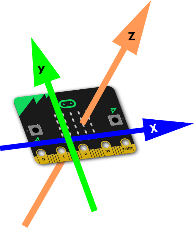
## micro:bit XYZ Planes and Orientation
---
## Flashing to micro:bit using Web Based Text Editor
[Python micro:bit Web Editor](https://python.microbit.org/v/3)
Click `Send to micro:bit`.

Follow instructions on screen.

Connect to micro:bit.

---
## Visualing the micro:bit Data via USB Cable
### Serial Port Writer main.py
This script is flashed onto the BBC micro:bit
```py
from microbit import *
while True:
sleep(100) # milliseconds
print(accelerometer.get_values())
```
The `print` command outputs to the USB serial port to be picked up by the connected laptop or computer.
### Serial Port Reader and Realtime Visualiser
**Imports:**
```py
from matplotlib import pyplot as plt
from matplotlib import animation
from numpy import diff
import serial
```
**Configuration:**
These constants define the serial port to attempt a connection to, the [Baud Rate](https://en.wikipedia.org/wiki/Baud) of the board, the timeout bit, the number of datapoints to display at a time and the rate at which the plot will update.
$$\text{LIMIT} \times \text{RATE} = \text{Number of Seconds Displayed}$$
*The Baud Rate to use can be found or changed in the Device Manager.*

```py
# Windows Device Manager > Ports (COM & LPT) > "mbed Serial Port"
PORT = 'COM3'
BAUD_RATE = 115_200 # ENSURE THIS MATCHES VALUE IN DEVICE MANAGER
STOP = 1
LIMIT = 300
RATE = 50 # ms
```
**Connect to Serial Port:**
Create a connection to the board. If the connection fails to open, exit the program.
```py
ser = serial.Serial(PORT, BAUD_RATE, timeout=STOP)
ser.close()
ser.open()
```
**Create Figure to Plot:**
Create a figure and add a subplot at position `111`.
```py
fig = plt.figure()
ax = fig.add_subplot(1, 1, 1)
```
**Initialise Lists for x, y and z Data:**
```py
xs, ys, zs = [0]*LIMIT, [0]*LIMIT, [0]*LIMIT
```
**Animate Function:**
Create the function `animate` that will get called as an argument in `FuncAnimate` later.
Read the line from the serial port connection. This is returned as a `byte` object so needs to be decoded with `.decode("utf-8")`. The parenthesis also need to be removed with `.strip()`. Then, cast the values to ints.
Create a list `idx` with length `LIMIT`. Append the current values to `xs`, `ys` and `zs`. Then, slice the list to only include the `n` most recent values, where `n` is `LIMIT`.
Calculate the deltas using `Numpy`'s `diff()` function. Then, plot the data and the deltas.
Once the lists have enough values in them, begin plotting.
```py
def animate(i, xs, ys, zs):
line = ser.readline().decode("utf-8").strip("(").strip(")\r\n")
x, y, z = line.split(",")
x, y, z = int(x), int(y), int(z)
print(x, y, z)
idx = range(LIMIT)
xs.append(x)
ys.append(y)
zs.append(z)
xs = xs[-LIMIT:]
ys = ys[-LIMIT:]
zs = zs[-LIMIT:]
d_xs = diff(xs)
d_ys = diff(ys)
d_zs = diff(zs)
if len(xs) == LIMIT:
ax.clear()
d_ax.clear()
ax.plot(idx, xs, color="r", label="X")
ax.plot(idx, ys, color="g", label="Y")
ax.plot(idx, zs, color="b", label="Z")
d_ax.plot(d_idx, d_xs, color="r")
d_ax.plot(d_idx, d_ys, color="g")
d_ax.plot(d_idx, d_zs, color="b")
d_ax.axhline(0, color="k")
ax.set_ylim(-1500, 1500)
d_ax.set_ylim(-1500, 1500)
ax.legend()
fig.suptitle("micro:bit Data Logger")
```
**Create and Plot Animation:**
Create the animation. This will call the `FuncAnimation` `animate` with arguments `xs`, `ys` and `zs` every `RATE` milliseconds. This occurs until the user causes a `KeyboardInterrupt` exception with Ctrl+C.
```py
ani = animation.FuncAnimation(
fig,
animate, fargs=(xs, ys, zs),
interval=RATE )
plt.show()
try:
pass
except KeyboardInterrupt:
ser.close()
```
### Serial Port Reader and 3D Realtime Visualiser
A lot of this code is repeated from the 2D visualiser. Some exceptions include:
- `RATE` and `LIMIT` values
- I had to increase the `RATE` constant (which decreases the rate - 1/n) and decrease the `LIMIT` constant which controls how many datapoints are displayed in order to avoid overloading the animation function. Even now, eventually the animation falls out of sync with the micro:bit's movements.
- `ax = plt.axes(projection='3d')`
- Creates a 3D Axis to plot data on.
- `ax.plot3D(xs, ys, zs)`
- Creates a line plot with `xs`, `ys` and `zs` as data inputs.
```py
from matplotlib import pyplot as plt
from matplotlib import animation
from numpy import diff
import serial
# Windows Device Manager > Ports (COM & LPT) > "mbed Serial Port"
PORT = 'COM3'
BAUD_RATE = 115_200 # ENSURE THIS MATCHES VALUE IN DEVICE MANAGER
STOP = 1
LIMIT = 25
RATE = 5 # ms
ser = serial.Serial(PORT, BAUD_RATE, timeout=STOP)
ser.close()
ser.open()
fig = plt.figure()
ax = plt.axes(projection='3d')
xs, ys, zs = [0]*LIMIT, [0]*LIMIT, [0]*LIMIT
def animate(i, xs, ys, zs):
line = ser.readline().decode("utf-8").strip("(").strip(")\r\n")
x, y, z = line.split(",")
x, y, z = int(x), int(y), int(z)
print(x, y, z)
idx = range(LIMIT)
xs.append(x)
ys.append(y)
zs.append(z)
xs = xs[-LIMIT:]
ys = ys[-LIMIT:]
zs = zs[-LIMIT:]
d_xs = diff(xs)
d_ys = diff(ys)
d_zs = diff(zs)
if len(xs) == LIMIT:
ax.clear()
ax.plot3D(xs, ys, zs, label="State")
ax.plot3D(d_xs, d_ys, d_zs, label="Deltas")
ax.set_xlim(-1500, 1500)
ax.set_ylim(-1500, 1500)
ax.set_zlim(-1500, 1500)
ax.legend()
ax.plot3D([-1500, 1500], [0, 0], [0, 0], "k--", alpha=0.5)
ax.plot3D([0, 0], [-1500, 1500], [0, 0], "k--", alpha=0.5)
ax.plot3D([0, 0], [0, 0], [-1500, 1500], "k--", alpha=0.5)
ani = animation.FuncAnimation(
fig,
animate, fargs=(xs, ys, zs),
interval=RATE )
plt.show()
try:
pass
except KeyboardInterrupt:
ser.close()
```
---
## Visualing the micro:bit with CSV Data
### Process
1. Run the data logger via battery power.
2. When you use the data logging feature on the micro:bit V2, an HTML file is created on the `MICROBIT` drive called `MY_DATA` that lets you interact with the logged data.
3. View `MY_DATA` in your browser. The page displays a set of buttons to interact with the data and a table containing the data that has been logged so far.
4. Click the Download button. This downloads the data in `.csv` format using a period `.` as the delimiter.
5. Run the `/not_connected/visualiser.py` script and follow any instructions that appear on screen.
### CSV Data Writer main.py
**Imports:**
```py
from microbit import *
import log, os
```
**Initialise the columns to log to:**
```py
# Set up columns for logging
log.set_labels('x', 'y', 'z')
```
**Define the `logger` function:**
This is the function that records the `x`, `y` and `z` values from the accelerometer into `"MY_DATA.HTM"`.
```py
# Record the x, y, z values
def logger():
log.add({
'x': accelerometer.get_x(),
'y': accelerometer.get_y(),
'z': accelerometer.get_z()
})
```
**Main Loop:**
The script begins by initialising `logging` to be `False`. Then, every 50ms* it will question whether any buttons have been pressed.
> *50ms: assuming unchanged since time of writing; this value may be changed if the log storage fills too quickly.
If A has been pressed, `logging` is set to `True`.
If B has been pressed, `logging` is set to `False`.
If `logging` is set to `True`, the `logger()` function is called. Since this call is within the outer `while True` loop, this function can be called every ~50ms*.
> *50ms delay + Loop Runtime
```py
# Pre initialise 'logging' as False / OFF
logging = False
while True:
sleep(50) # milliseconds
# On "A" button pressed...
if button_a.is_pressed():
logging = True
display.show(Image.YES)
# On "B" button pressed...
# Set logging to False and update displayed icon
if button_b.is_pressed():
logging = False
display.show(Image.NO)
# If logging is set to True...
# Call the logging function and record values
if logging:
logger()
```
### CSV Data Visualiser
**Imports:**
```py
from tkinter import filedialog as fd
import pandas as pd
from matplotlib import pyplot as plt
from matplotlib.gridspec import GridSpec
from scipy import signal
```
**File Selection and Reading:**
Opens a File Explorer window allowing the user to select the `.csv` file to plot. This file is read into a `panda` `Dataframe` Object using a comma `,` as the delimiter. `.reset_index()` creates an `index` column which is used as the x-variable during plotting.
```py
file = fd.askopenfilename(
filetypes=[("CSV files", "*.csv")],title="Set input .csv file" )
data = pd.read_csv(file, header=0).reset_index()
```
**Create Figure:**
```py
fig = plt.figure(figsize=(10, 10))
gs = GridSpec(9, 6, figure=fig)
ax = fig.add_subplot(gs[0:3, 0:3])
d_ax = fig.add_subplot(gs[0:3, 3:6])
dx_ax = fig.add_subplot(gs[3:6, 0:2])
dy_ax = fig.add_subplot(gs[3:6, 2:4])
dz_ax = fig.add_subplot(gs[3:6, 4:6])
xpeak_ax = fig.add_subplot(gs[6:9, 0:2])
ypeak_ax = fig.add_subplot(gs[6:9, 2:4])
zpeak_ax = fig.add_subplot(gs[6:9, 4:6])
fig.tight_layout(pad=2.5)
ax.axhline(0, color="k")
d_ax.axhline(0, color="k")
dx_ax.axhline(0, color="k")
dy_ax.axhline(0, color="k")
dz_ax.axhline(0, color="k")
xpeak_ax.axhline(0, color="k")
ypeak_ax.axhline(0, color="k")
zpeak_ax.axhline(0, color="k")
```
**Calculate Rolling Average:**
```py
ROLLER = 4
ALPHA = 0.3
rolling = data.rolling(ROLLER).mean()
rolling = rolling.dropna().reset_index()
```
**Plot Data (Raw and Rolling Values):**
```py
# Plot the data
ax.plot(data.index, data.x, "r--", label="X", alpha=0.3)
ax.plot(data.index, data.y, "g--", label="Y", alpha=0.3)
ax.plot(data.index, data.z, "b--", label="Z", alpha=0.3)
# Plot rolling average data
ax.plot(rolling.index + ROLLER/2, rolling.x, "r", label="X")
ax.plot(rolling.index + ROLLER/2, rolling.y, "g", label="Y")
ax.plot(rolling.index + ROLLER/2, rolling.z, "b", label="Z")
```
**Calculate Deltas:**
```py
# Calculate deltas
data['dx'] = data['x'] - data['x'].shift(-1)
data['dy'] = data['y'] - data['y'].shift(-1)
data['dz'] = data['z'] - data['z'].shift(-1)
rolling['dx'] = rolling['x'] - rolling['x'].shift(-1)
rolling['dy'] = rolling['y'] - rolling['y'].shift(-1)
rolling['dz'] = rolling['z'] - rolling['z'].shift(-1)
```
**Plot Deltas (Raw and Rolling Values):**:
```py
# Plot deltas
d_ax.plot(data.index, data.dx, "r--", label="X", alpha=0.3)
d_ax.plot(data.index, data.dy, "g--", label="Y", alpha=0.3)
d_ax.plot(data.index, data.dz, "b--", label="Z", alpha=0.3)
# Plot rolling deltas shifted to align with the 'data' values
d_ax.plot(rolling.index + ROLLER/2, rolling.dx, "r", label="X")
d_ax.plot(rolling.index + ROLLER/2, rolling.dy, "g", label="Y")
d_ax.plot(rolling.index + ROLLER/2, rolling.dz, "b", label="Z")
```
**Plot Deltas Seperately:**
This is done on both the `dn_ax` and the `npeak_ax` axis'.
```py
dx_ax.plot(data.index, data.dx, "r--", label="X", alpha=ALPHA)
dy_ax.plot(data.index, data.dy, "g--", label="Y", alpha=ALPHA)
dz_ax.plot(data.index, data.dz, "b--", label="Z", alpha=ALPHA)
dx_ax.plot(rolling.index + ROLLER/2, rolling.dx, "r", label="X")
dy_ax.plot(rolling.index + ROLLER/2, rolling.dy, "g", label="Y")
dz_ax.plot(rolling.index + ROLLER/2, rolling.dz, "b", label="Z")
xpeak_ax.plot(data.index, data.dx, "r--", label="X", alpha=ALPHA)
ypeak_ax.plot(data.index, data.dy, "g--", label="Y", alpha=ALPHA)
zpeak_ax.plot(data.index, data.dz, "b--", label="Z", alpha=ALPHA)
xpeak_ax.plot(rolling.index + ROLLER/2, rolling.dx, "r", label="X")
ypeak_ax.plot(rolling.index + ROLLER/2, rolling.dy, "g", label="Y")
zpeak_ax.plot(rolling.index + ROLLER/2, rolling.dz, "b", label="Z")
```
**Format the Plot:**
Find the highest magnitude values (positive or negative) for the `x`, `y` and `z` as well as the `dx`, `dy` and `dz` columns of `rolling`. Use these +50% as the y-limits for the axis. The added percentage ensures the data is not crowded with the axis borders.
```py
# Find max x, y, z magnitude for rolling data, then +50% as leeway
ax_bound = abs( rolling[["x","y","z"]] ).max().max() * 1.5
ax.set_ylim(-ax_bound, ax_bound)
# Find max x, y, z magnitude for rolling deltas, then +50% as leeway
d_bound = abs( rolling[["dx","dy","dz"]] ).max().max() * 1.5
d_ax.set_ylim(-d_bound, d_bound)
# Find max x, y, z magnitude for rolling deltas, then +10% as leeway
peak_bound = abs( rolling[["dx","dy","dz"]] ).max().max() * 1.1
# Set titles and create legends
fig.suptitle("micro:bit Data Logger")
ax.set_title("Raw Data")
d_ax.set_title("Deltas")
dx_ax.set_title("dx")
dy_ax.set_title("dy")
dz_ax.set_title("dz")
xpeak_ax.set_title("x_peaks")
ypeak_ax.set_title("y_peaks")
zpeak_ax.set_title("z_peaks")
dx_ax.set_ylim(-d_bound, d_bound)
dy_ax.set_ylim(-d_bound, d_bound)
dz_ax.set_ylim(-d_bound, d_bound)
ax.legend()
d_ax.legend()
```
**Plot Peaks:**
Plot vertical lines at signal peaks +/- 20; this signifies the zone cropped into on the lower plots.
```py
from scipy import signal
THRESHOLD = 200
x_peaks, x_props = signal.find_peaks(rolling.dx, threshold=THRESHOLD)
y_peaks, y_props = signal.find_peaks(rolling.dy, threshold=THRESHOLD)
z_peaks, z_props = signal.find_peaks(rolling.dz, threshold=THRESHOLD)
# This function plots vertical lines on each of the seperated delta plots to
# indicate which section of the data is being cropped into on
# the proceeding plot.
# It then crops into these areas
# If no peaks are found it will delete that subplot.
def plot_peaks(delta_axis, peak_axis, peaks):
try:
delta_axis.axvline(peaks[0] - 20, color="k", alpha=0.7)
delta_axis.axvline(peaks[0] + 20, color="k", alpha=0.7)
# Set the x and y bounds for each of the peak plots
peak_axis.set_xlim(peaks[len(peaks)//2] - 20, peaks[len(peaks)//2] + 20)
peak_axis.set_ylim(-peak_bound, peak_bound)
except IndexError:
print("No peaks found...")
print(peaks)
fig.delaxes(peak_axis)
plot_peaks(dx_ax, xpeak_ax, x_peaks)
plot_peaks(dy_ax, ypeak_ax, y_peaks)
plot_peaks(dz_ax, zpeak_ax, z_peaks)
```
**Crop into peaks:**
Use the 'middle index' peak to decide where to crop into.
```py
xpeak_ax.set_xlim(x_peaks[len(x_peaks)//2] - 20, x_peaks[len(x_peaks)//2] + 20)
ypeak_ax.set_xlim(y_peaks[len(y_peaks)//2] - 20, y_peaks[len(y_peaks)//2] + 20)
zpeak_ax.set_xlim(z_peaks[len(z_peaks)//2] - 20, z_peaks[len(z_peaks)//2] + 20)
xpeak_ax.set_ylim(-peak_bound, peak_bound)
ypeak_ax.set_ylim(-peak_bound, peak_bound)
zpeak_ax.set_ylim(-peak_bound, peak_bound)
```
> Uses integer division.
```
>>> 1//2
0
>>> 2//2
1
>>> 3//2
1
>>> 4//2
2
```
### CSV Data 3D Visualiser
**Imports:**
```py
from tkinter import filedialog as fd
import pandas as pd
import matplotlib.pyplot as plt
```
**File Selection and Reading:**
Opens a File Explorer window allowing the user to select the `.csv` file to plot. This file is read into a `panda` `Dataframe` Object using a comma `,` as the delimiter. `.reset_index()` creates an `index` column which is used as the x-variable during plotting.
```py
file = fd.askopenfilename(
filetypes=[("CSV files", "*.csv")],title="Set input .csv file" )
data = pd.read_csv(file, header=0, delimiter=",")
```
**Create 3D Plot:**
Create the figure `fig` and 3D axis `ax`. Plot the data as a continuous line showing the movement of the micro:bit.
```py
fig = plt.figure()
ax = plt.axes(projection='3d')
ax.plot3D(x, y, z, color='k')
ax.set_xlim(-1500, 1500)
ax.set_ylim(-1500, 1500)
ax.set_zlim(-1500, 1500)
ax.plot3D([-1500, 1500], [0, 0], [0, 0], "k--", alpha=0.5)
ax.plot3D([0, 0], [-1500, 1500], [0, 0], "k--", alpha=0.5)
ax.plot3D([0, 0], [0, 0], [-1500, 1500], "k--", alpha=0.5)
plt.show()
```
---
## Output
### Serial Port Connection


### From CSV Data


---
## Final Project and Presentation
An interesting scenario to record could be archery. This would show how movement / stabilisation changes throughout the shot process and the vibrations and forces involved during the loose of an arrow. This would be similar to a commercial product called the "Mantis X8 Archery Training Tool for Marksmanship" which measures shot feedback, allowing the archer to visualise movements that the human eye will not see.
### Project Selection
Archery Stability Tracker: Measure the vibrations of a bow as it is fired. This could also be used to visualise different stages of the shot process; nocking, setting, aiming, loosing.
This could also be used to compare other variables:
- Bowstyle: Recurve Vs. Compound
- Vibration Dampening: With and without 'Limb Savers'
- Distance: Do I aim / settle for longer at higher distances?
### Plan
- Write a script for the micro:bit to record accelerometer data in `.csv` format every `n` milliseconds.
- When Button "A" is pressed, start recording; would it be a good idea to include a 2-3 second delay to avoid recording 'interference'? If so, will need a visual indication and / or countdown.
- When Button "B" is pressed, stop recording.
- Carry out signal pre-processing to mitigate random noise. This could be carried out with methods such as convolving (rolling averages) or even Kalman filtering.
- Use Python's `matplotlib` module to visualise the movement in various formats: 2D and 3D lineplot.
- Use Python's `matplotlib` module to visualise the rate of movement (deltas between datapoints).
- Focus in on 'spikes' within the data, likely to be the moment of loosing.
> DEFINITION - Loosing: The act of shooting an arrow from a bow.
### Why?
I will be using `.csv` data in this project as opposed to serial port transfer between the micro:bit and a computer as this would allow the micro:bit to be a small and standalone unit; a long cable connecting two devices would pose a safety hazard if the wire got caught in the cam system of my compound bow.
> DEFINITION - Cam System: Pulley/s on the limbs of the bow that 'hold' the draw weight at full draw. This allows you to hold a heavy draw weight as though it was a light draw weight meaning you can stay at a settled full draw for an extended time period. Or, a rotating piece of mechanical linkage that converts rotary motion into linear motion.
Real-time logging could be achieved using the `radio` functionality of *two* micro:bits; one on the bow to record and transmit the data and on connected to a computer / laptop to receive and plot. This is demonstrated in [this](https://microbit.org/projects/make-it-code-it/python-wireless-data-logger/) project.
### What Went Well
### Lessons Learned
### Testing and Results
### Potential Application
---