https://github.com/coreyjs/face-generation-gan
A GAN to generate human faces.
https://github.com/coreyjs/face-generation-gan
Last synced: 4 months ago
JSON representation
A GAN to generate human faces.
- Host: GitHub
- URL: https://github.com/coreyjs/face-generation-gan
- Owner: coreyjs
- Created: 2021-03-27T20:23:23.000Z (over 5 years ago)
- Default Branch: master
- Last Pushed: 2021-03-27T20:26:39.000Z (over 5 years ago)
- Last Synced: 2025-08-05T23:28:46.948Z (11 months ago)
- Language: HTML
- Size: 1.27 MB
- Stars: 1
- Watchers: 1
- Forks: 0
- Open Issues: 1
-
Metadata Files:
- Readme: README.md
Awesome Lists containing this project
README
# face-generation-GAN
A GAN to generate human faces.
# Face Generation
In this project, you'll define and train a DCGAN on a dataset of faces. Your goal is to get a generator network to generate *new* images of faces that look as realistic as possible!
The project will be broken down into a series of tasks from **loading in data to defining and training adversarial networks**. At the end of the notebook, you'll be able to visualize the results of your trained Generator to see how it performs; your generated samples should look like fairly realistic faces with small amounts of noise.
### Get the Data
You'll be using the [CelebFaces Attributes Dataset (CelebA)](http://mmlab.ie.cuhk.edu.hk/projects/CelebA.html) to train your adversarial networks.
This dataset is more complex than the number datasets (like MNIST or SVHN) you've been working with, and so, you should prepare to define deeper networks and train them for a longer time to get good results. It is suggested that you utilize a GPU for training.
### Pre-processed Data
Since the project's main focus is on building the GANs, we've done *some* of the pre-processing for you. Each of the CelebA images has been cropped to remove parts of the image that don't include a face, then resized down to 64x64x3 NumPy images. Some sample data is show below.

> If you are working locally, you can download this data [by clicking here](https://s3.amazonaws.com/video.udacity-data.com/topher/2018/November/5be7eb6f_processed-celeba-small/processed-celeba-small.zip)
This is a zip file that you'll need to extract in the home directory of this notebook for further loading and processing. After extracting the data, you should be left with a directory of data `processed_celeba_small/`
```python
# can comment out after executing
!unzip processed_celeba_small.zip
```
'unzip' is not recognized as an internal or external command,
operable program or batch file.
```python
data_dir = 'processed_celeba_small/'
"""
DON'T MODIFY ANYTHING IN THIS CELL
"""
import pickle as pkl
import matplotlib.pyplot as plt
import numpy as np
import problem_unittests as tests
#import helper
%matplotlib inline
```
## Visualize the CelebA Data
The [CelebA](http://mmlab.ie.cuhk.edu.hk/projects/CelebA.html) dataset contains over 200,000 celebrity images with annotations. Since you're going to be generating faces, you won't need the annotations, you'll only need the images. Note that these are color images with [3 color channels (RGB)](https://en.wikipedia.org/wiki/Channel_(digital_image)#RGB_Images) each.
### Pre-process and Load the Data
Since the project's main focus is on building the GANs, we've done *some* of the pre-processing for you. Each of the CelebA images has been cropped to remove parts of the image that don't include a face, then resized down to 64x64x3 NumPy images. This *pre-processed* dataset is a smaller subset of the very large CelebA data.
> There are a few other steps that you'll need to **transform** this data and create a **DataLoader**.
#### Exercise: Complete the following `get_dataloader` function, such that it satisfies these requirements:
* Your images should be square, Tensor images of size `image_size x image_size` in the x and y dimension.
* Your function should return a DataLoader that shuffles and batches these Tensor images.
#### ImageFolder
To create a dataset given a directory of images, it's recommended that you use PyTorch's [ImageFolder](https://pytorch.org/docs/stable/torchvision/datasets.html#imagefolder) wrapper, with a root directory `processed_celeba_small/` and data transformation passed in.
```python
# necessary imports
import torch
import os
from torchvision import datasets
from torchvision import transforms
from torch.utils.data import DataLoader
```
```python
def get_dataloader(batch_size, image_size, data_dir='processed_celeba_small/') -> DataLoader:
"""
Batch the neural network data using DataLoader
:param batch_size: The size of each batch; the number of images in a batch
:param img_size: The square size of the image data (x, y)
:param data_dir: Directory where image data is located
:return: DataLoader with batched data
"""
# TODO: Implement function and return a dataloader
# resize and normalize the images (variation of code found in CycleGAN notebook)
t = transforms.Compose([
transforms.Resize(image_size),
transforms.ToTensor()
])
dataset = datasets.ImageFolder(data_dir, transform=t)
loader = DataLoader(
dataset=dataset,
batch_size=batch_size,
shuffle=True
)
return loader
```
## Create a DataLoader
#### Exercise: Create a DataLoader `celeba_train_loader` with appropriate hyperparameters.
Call the above function and create a dataloader to view images.
* You can decide on any reasonable `batch_size` parameter
* Your `image_size` **must be** `32`. Resizing the data to a smaller size will make for faster training, while still creating convincing images of faces!
```python
# Define function hyperparameters
batch_size = 128
img_size = 32
"""
DON'T MODIFY ANYTHING IN THIS CELL THAT IS BELOW THIS LINE
"""
# Call your function and get a dataloader
celeba_train_loader = get_dataloader(batch_size, img_size)
```
Next, you can view some images! You should seen square images of somewhat-centered faces.
Note: You'll need to convert the Tensor images into a NumPy type and transpose the dimensions to correctly display an image, suggested `imshow` code is below, but it may not be perfect.
```python
# helper display function
def imshow(img):
npimg = img.numpy()
plt.imshow(np.transpose(npimg, (1, 2, 0)))
"""
DON'T MODIFY ANYTHING IN THIS CELL THAT IS BELOW THIS LINE
"""
# obtain one batch of training images
dataiter = iter(celeba_train_loader)
images, _ = dataiter.next() # _ for no labels
# plot the images in the batch, along with the corresponding labels
fig = plt.figure(figsize=(20, 4))
plot_size=20
for idx in np.arange(plot_size):
ax = fig.add_subplot(2, plot_size/2, idx+1, xticks=[], yticks=[])
imshow(images[idx])
```
C:\Users\cscha\anaconda3\envs\u-deep-learning\lib\site-packages\ipykernel_launcher.py:17: MatplotlibDeprecationWarning: Passing non-integers as three-element position specification is deprecated since 3.3 and will be removed two minor releases later.

#### Exercise: Pre-process your image data and scale it to a pixel range of -1 to 1
You need to do a bit of pre-processing; you know that the output of a `tanh` activated generator will contain pixel values in a range from -1 to 1, and so, we need to rescale our training images to a range of -1 to 1. (Right now, they are in a range from 0-1.)
```python
# TODO: Complete the scale function
def scale(x, feature_range=(-1, 1)):
''' Scale takes in an image x and returns that image, scaled
with a feature_range of pixel values from -1 to 1.
This function assumes that the input x is already scaled from 0-1.'''
# assume x is scaled to (0, 1)
# scale to feature_range and return scaled x
# unpack tuple
min, max = feature_range
x = x * (max - min) + min
return x
```
```python
"""
DON'T MODIFY ANYTHING IN THIS CELL THAT IS BELOW THIS LINE
"""
# check scaled range
# should be close to -1 to 1
img = images[0]
print('Orig Min: ', img.min())
print('Orig Max: ', img.max())
scaled_img = scale(img)
print('Min: ', scaled_img.min())
print('Max: ', scaled_img.max())
```
Orig Min: tensor(0.0784)
Orig Max: tensor(1.)
Min: tensor(-0.8431)
Max: tensor(1.)
---
# Define the Model
A GAN is comprised of two adversarial networks, a discriminator and a generator.
## Discriminator
Your first task will be to define the discriminator. This is a convolutional classifier like you've built before, only without any maxpooling layers. To deal with this complex data, it's suggested you use a deep network with **normalization**. You are also allowed to create any helper functions that may be useful.
#### Exercise: Complete the Discriminator class
* The inputs to the discriminator are 32x32x3 tensor images
* The output should be a single value that will indicate whether a given image is real or fake
```python
import torch.nn as nn
import torch.nn.functional as F
```
```python
# Helper Functions
# Similar to those in chapter 5
def get_conv_layers(in_channels, out_channels, kernel_size, stride=2, padding=1, batch_norm=True):
"""
This will create a conv layer with optional batch norm applied
"""
layers = []
layers.append(
nn.Conv2d(
in_channels=in_channels,
out_channels=out_channels,
kernel_size=kernel_size,
stride=stride,
padding=padding,
bias=False
)
)
if batch_norm:
layers.append(nn.BatchNorm2d(out_channels))
return nn.Sequential(*layers)
```
```python
class Discriminator(nn.Module):
def __init__(self, conv_dim):
"""
Initialize the Discriminator Module
:param conv_dim: The depth of the first convolutional layer
"""
super(Discriminator, self).__init__()
# complete init function
# we will define a 4 layer network due to the small input size of our images
self.conv_dim = conv_dim
# x, y = 32, depth 32
# Note, first layer does not have batch normilization
self.conv1 = get_conv_layers(
in_channels=3, #rgb
out_channels=conv_dim,
kernel_size=4,
batch_norm=False
)
# (16, 16, 64)
self.conv2 = get_conv_layers(
in_channels=conv_dim,
out_channels=conv_dim*2,
kernel_size=4
)
# (8, 8, 128)
self.conv3 = get_conv_layers(
in_channels=conv_dim * 2,
out_channels=conv_dim * 4,
kernel_size=4
)
self.fc = nn.Linear(conv_dim * 4 * 4 * 4, 1)
def forward(self, x):
"""
Forward propagation of the neural network
:param x: The input to the neural network
:return: Discriminator logits; the output of the neural network
"""
# define feedforward behavior
out = F.leaky_relu(self.conv1(x), 0.2)
out = F.leaky_relu(self.conv2(out), 0.2)
out = F.leaky_relu(self.conv3(out), 0.2)
# flatten image
out = out.view(-1, self.conv_dim*4*4*4)
#final output layer
out = self.fc(out)
return out
"""
DON'T MODIFY ANYTHING IN THIS CELL THAT IS BELOW THIS LINE
"""
tests.test_discriminator(Discriminator)
```
Tests Passed
## Generator
The generator should upsample an input and generate a *new* image of the same size as our training data `32x32x3`. This should be mostly transpose convolutional layers with normalization applied to the outputs.
#### Exercise: Complete the Generator class
* The inputs to the generator are vectors of some length `z_size`
* The output should be a image of shape `32x32x3`

```python
# helper method
def get_deconv_layers(in_channels, out_channels, kernel_size, stride=2, padding=1, batch_norm=True):
"""
This will create a transposed convultional layer, with optional batch normilization.
"""
layers = []
layers.append(
nn.ConvTranspose2d(
in_channels=in_channels,
out_channels=out_channels,
kernel_size=kernel_size,
stride=stride,
padding=padding,
bias=False
)
)
if batch_norm:
layers.append(nn.BatchNorm2d(out_channels))
return nn.Sequential(*layers)
```
```python
class Generator(nn.Module):
def __init__(self, z_size, conv_dim):
"""
Initialize the Generator Module
:param z_size: The length of the input latent vector, z
:param conv_dim: The depth of the inputs to the *last* transpose convolutional layer
"""
super(Generator, self).__init__()
# complete init function
self.conv_dim = conv_dim
# following previous generator examples, we will start with a
# fullconnected (fc) layer, followed by 3 transpose conv layers
# and finally out outputed, generated image
self.fc = nn.Linear(z_size, conv_dim*4*4*4)
self.t_conv1 = get_deconv_layers(
in_channels=conv_dim * 4,
out_channels=conv_dim *2,
kernel_size=4
)
self.t_conv2 = get_deconv_layers(
in_channels=conv_dim *2,
out_channels=conv_dim,
kernel_size=4
)
self.t_conv3 = get_deconv_layers(
in_channels=conv_dim,
out_channels=3,
kernel_size=4,
batch_norm=False
)
def forward(self, x):
"""
Forward propagation of the neural network
:param x: The input to the neural network
:return: A 32x32x3 Tensor image as output
"""
# define feedforward behavior
out = self.fc(x)
# reshape
out = out.view(-1, self.conv_dim*4, 4, 4) # (batchsize, depth, 4, 4)
out = F.relu(self.t_conv1(out))
out = F.relu(self.t_conv2(out))
# final layert and activation
out = self.t_conv3(out)
out = F.tanh(out) # F.tanh is deprecated
return out
"""
DON'T MODIFY ANYTHING IN THIS CELL THAT IS BELOW THIS LINE
"""
tests.test_generator(Generator)
```
Tests Passed
C:\Users\cscha\anaconda3\envs\u-deep-learning\lib\site-packages\torch\nn\functional.py:1628: UserWarning: nn.functional.tanh is deprecated. Use torch.tanh instead.
warnings.warn("nn.functional.tanh is deprecated. Use torch.tanh instead.")
## Initialize the weights of your networks
To help your models converge, you should initialize the weights of the convolutional and linear layers in your model. From reading the [original DCGAN paper](https://arxiv.org/pdf/1511.06434.pdf), they say:
> All weights were initialized from a zero-centered Normal distribution with standard deviation 0.02.
So, your next task will be to define a weight initialization function that does just this!
You can refer back to the lesson on weight initialization or even consult existing model code, such as that from [the `networks.py` file in CycleGAN Github repository](https://github.com/junyanz/pytorch-CycleGAN-and-pix2pix/blob/master/models/networks.py) to help you complete this function.
#### Exercise: Complete the weight initialization function
* This should initialize only **convolutional** and **linear** layers
* Initialize the weights to a normal distribution, centered around 0, with a standard deviation of 0.02.
* The bias terms, if they exist, may be left alone or set to 0.
```python
def weights_init_normal(m):
"""
Applies initial weights to certain layers in a model .
The weights are taken from a normal distribution
with mean = 0, std dev = 0.02.
:param m: A module or layer in a network
"""
# classname will be something like:
# `Conv`, `BatchNorm2d`, `Linear`, etc.
classname = m.__class__.__name__
# referenced from https://github.com/junyanz/pytorch-CycleGAN-and-pix2pix/blob/master/models/networks.py
if hasattr(m, 'weight') and (classname.find('Conv') != -1 or classname.find('Linear') != -1):
m.weight.data.normal_(0.0, 0.02)
if hasattr(m, 'bias') and m.bias is not None:
m.bias.data.zero_()
```
## Build complete network
Define your models' hyperparameters and instantiate the discriminator and generator from the classes defined above. Make sure you've passed in the correct input arguments.
```python
"""
DON'T MODIFY ANYTHING IN THIS CELL THAT IS BELOW THIS LINE
"""
def build_network(d_conv_dim, g_conv_dim, z_size):
# define discriminator and generator
D = Discriminator(d_conv_dim)
G = Generator(z_size=z_size, conv_dim=g_conv_dim)
# initialize model weights
D.apply(weights_init_normal)
G.apply(weights_init_normal)
print(D)
print()
print(G)
return D, G
```
#### Exercise: Define model hyperparameters
```python
# Define model hyperparams
d_conv_dim = 64
g_conv_dim = 64
z_size = 100
"""
DON'T MODIFY ANYTHING IN THIS CELL THAT IS BELOW THIS LINE
"""
D, G = build_network(d_conv_dim, g_conv_dim, z_size)
```
Discriminator(
(conv1): Sequential(
(0): Conv2d(3, 64, kernel_size=(4, 4), stride=(2, 2), padding=(1, 1), bias=False)
)
(conv2): Sequential(
(0): Conv2d(64, 128, kernel_size=(4, 4), stride=(2, 2), padding=(1, 1), bias=False)
(1): BatchNorm2d(128, eps=1e-05, momentum=0.1, affine=True, track_running_stats=True)
)
(conv3): Sequential(
(0): Conv2d(128, 256, kernel_size=(4, 4), stride=(2, 2), padding=(1, 1), bias=False)
(1): BatchNorm2d(256, eps=1e-05, momentum=0.1, affine=True, track_running_stats=True)
)
(fc): Linear(in_features=4096, out_features=1, bias=True)
)
Generator(
(fc): Linear(in_features=100, out_features=4096, bias=True)
(t_conv1): Sequential(
(0): ConvTranspose2d(256, 128, kernel_size=(4, 4), stride=(2, 2), padding=(1, 1), bias=False)
(1): BatchNorm2d(128, eps=1e-05, momentum=0.1, affine=True, track_running_stats=True)
)
(t_conv2): Sequential(
(0): ConvTranspose2d(128, 64, kernel_size=(4, 4), stride=(2, 2), padding=(1, 1), bias=False)
(1): BatchNorm2d(64, eps=1e-05, momentum=0.1, affine=True, track_running_stats=True)
)
(t_conv3): Sequential(
(0): ConvTranspose2d(64, 3, kernel_size=(4, 4), stride=(2, 2), padding=(1, 1), bias=False)
)
)
### Training on GPU
Check if you can train on GPU. Here, we'll set this as a boolean variable `train_on_gpu`. Later, you'll be responsible for making sure that
>* Models,
* Model inputs, and
* Loss function arguments
Are moved to GPU, where appropriate.
```python
"""
DON'T MODIFY ANYTHING IN THIS CELL
"""
import torch
# Check for a GPU
train_on_gpu = torch.cuda.is_available()
if not train_on_gpu:
print('No GPU found. Please use a GPU to train your neural network.')
else:
print('Training on GPU!')
```
Training on GPU!
---
## Discriminator and Generator Losses
Now we need to calculate the losses for both types of adversarial networks.
### Discriminator Losses
> * For the discriminator, the total loss is the sum of the losses for real and fake images, `d_loss = d_real_loss + d_fake_loss`.
* Remember that we want the discriminator to output 1 for real images and 0 for fake images, so we need to set up the losses to reflect that.
### Generator Loss
The generator loss will look similar only with flipped labels. The generator's goal is to get the discriminator to *think* its generated images are *real*.
#### Exercise: Complete real and fake loss functions
**You may choose to use either cross entropy or a least squares error loss to complete the following `real_loss` and `fake_loss` functions.**
```python
def real_loss(D_out):
'''Calculates how close discriminator outputs are to being real.
param, D_out: discriminator logits
return: real loss'''
batch_size = D_out.size(0)
labels = torch.ones(batch_size)
if train_on_gpu:
labels = labels.cuda()
# binary cross entropy loss with logits loss
criterion = nn.BCEWithLogitsLoss()
loss = criterion(D_out.squeeze(), labels)
return loss
def fake_loss(D_out):
'''Calculates how close discriminator outputs are to being fake.
param, D_out: discriminator logits
return: fake loss'''
batch_size = D_out.size(0)
labels = torch.zeros(batch_size)
if train_on_gpu:
labels = labels.cuda()
criterion = nn.BCEWithLogitsLoss()
loss = criterion(D_out.squeeze(), labels)
return loss
```
## Optimizers
#### Exercise: Define optimizers for your Discriminator (D) and Generator (G)
Define optimizers for your models with appropriate hyperparameters.
```python
import torch.optim as optim
lr = 0.0002 #0.0002
beta1 = 0.5
beta2 = 0.999
# Create optimizers for the discriminator D and generator G
d_optimizer = optim.Adam(D.parameters(), lr, [beta1, beta2])
g_optimizer = optim.Adam(G.parameters(), lr, [beta1, beta2])
```
---
## Training
Training will involve alternating between training the discriminator and the generator. You'll use your functions `real_loss` and `fake_loss` to help you calculate the discriminator losses.
* You should train the discriminator by alternating on real and fake images
* Then the generator, which tries to trick the discriminator and should have an opposing loss function
#### Saving Samples
You've been given some code to print out some loss statistics and save some generated "fake" samples.
#### Exercise: Complete the training function
Keep in mind that, if you've moved your models to GPU, you'll also have to move any model inputs to GPU.
```python
def train(D, G, n_epochs, print_every=50):
'''Trains adversarial networks for some number of epochs
param, D: the discriminator network
param, G: the generator network
param, n_epochs: number of epochs to train for
param, print_every: when to print and record the models' losses
return: D and G losses'''
# move models to GPU
if train_on_gpu:
D.cuda()
G.cuda()
# keep track of loss and generated, "fake" samples
samples = []
losses = []
# Get some fixed data for sampling. These are images that are held
# constant throughout training, and allow us to inspect the model's performance
sample_size=16
fixed_z = np.random.uniform(-1, 1, size=(sample_size, z_size))
fixed_z = torch.from_numpy(fixed_z).float()
# move z to GPU if available
if train_on_gpu:
fixed_z = fixed_z.cuda()
# epoch training loop
for epoch in range(n_epochs):
# batch training loop
for batch_i, (real_images, _) in enumerate(celeba_train_loader):
batch_size = real_images.size(0)
real_images = scale(real_images)
if train_on_gpu:
real_images = real_images.cuda()
# ===============================================
# YOUR CODE HERE: TRAIN THE NETWORKS
# ===============================================
# 1. Train the discriminator on real and fake images
d_optimizer.zero_grad()
# train with real images
d_real = D(real_images)
d_real_loss = real_loss(d_real)
# train with fake images
# referenced on DCGAN udacity notebook
z = np.random.uniform(-1, 1, size=(batch_size, z_size))
z = torch.from_numpy(z).float()
# move x to GPU, if available
if train_on_gpu:
z = z.cuda()
fake_images = G(z)
d_fake = D(fake_images)
d_fake_loss = fake_loss(d_fake)
# add up loss and do backprop
d_loss = d_real_loss + d_fake_loss
d_loss.backward()
d_optimizer.step()
# 2. Train the generator with an adversarial loss
g_optimizer.zero_grad()
#train with fake images and flipped labels
#gen fake images
z = np.random.uniform(-1, 1, size=(batch_size, z_size))
z = torch.from_numpy(z).float()
if train_on_gpu:
z = z.cuda()
fake_images = G(z)
# compute discrim losses on fake images
D_fake = D(fake_images)
g_loss = real_loss(D_fake)
#backprop
g_loss.backward()
g_optimizer.step()
# ===============================================
# END OF YOUR CODE
# ===============================================
# Print some loss stats
if batch_i % print_every == 0:
# append discriminator loss and generator loss
losses.append((d_loss.item(), g_loss.item()))
# print discriminator and generator loss
print('Epoch [{:5d}/{:5d}] | d_loss: {:6.4f} | g_loss: {:6.4f}'.format(
epoch+1, n_epochs, d_loss.item(), g_loss.item()))
## AFTER EACH EPOCH##
# this code assumes your generator is named G, feel free to change the name
# generate and save sample, fake images
G.eval() # for generating samples
samples_z = G(fixed_z)
samples.append(samples_z)
G.train() # back to training mode
# Save training generator samples
with open('train_samples.pkl', 'wb') as f:
pkl.dump(samples, f)
# finally return losses
return losses
```
Set your number of training epochs and train your GAN!
```python
# set number of epochs
n_epochs = 30
"""
DON'T MODIFY ANYTHING IN THIS CELL
"""
# call training function
losses = train(D, G, n_epochs=n_epochs)
```
C:\Users\cscha\anaconda3\envs\u-deep-learning\lib\site-packages\torch\nn\functional.py:1628: UserWarning: nn.functional.tanh is deprecated. Use torch.tanh instead.
warnings.warn("nn.functional.tanh is deprecated. Use torch.tanh instead.")
Epoch [ 1/ 30] | d_loss: 0.9295 | g_loss: 1.5117
Epoch [ 1/ 30] | d_loss: 1.0034 | g_loss: 1.8572
Epoch [ 1/ 30] | d_loss: 1.0981 | g_loss: 2.0010
Epoch [ 1/ 30] | d_loss: 0.8415 | g_loss: 1.8121
Epoch [ 2/ 30] | d_loss: 0.9711 | g_loss: 1.0954
Epoch [ 2/ 30] | d_loss: 0.7390 | g_loss: 2.1245
Epoch [ 2/ 30] | d_loss: 1.1486 | g_loss: 1.0666
Epoch [ 2/ 30] | d_loss: 0.9295 | g_loss: 1.3925
Epoch [ 3/ 30] | d_loss: 0.9660 | g_loss: 0.9416
Epoch [ 3/ 30] | d_loss: 0.8961 | g_loss: 1.6030
Epoch [ 3/ 30] | d_loss: 0.9145 | g_loss: 1.0857
Epoch [ 3/ 30] | d_loss: 1.0376 | g_loss: 0.9892
Epoch [ 4/ 30] | d_loss: 1.1725 | g_loss: 0.6244
Epoch [ 4/ 30] | d_loss: 1.1803 | g_loss: 0.8774
Epoch [ 4/ 30] | d_loss: 0.8313 | g_loss: 1.5151
Epoch [ 4/ 30] | d_loss: 0.8474 | g_loss: 1.7635
Epoch [ 5/ 30] | d_loss: 0.8062 | g_loss: 1.6507
Epoch [ 5/ 30] | d_loss: 0.8955 | g_loss: 1.4647
Epoch [ 5/ 30] | d_loss: 0.9882 | g_loss: 0.8468
Epoch [ 5/ 30] | d_loss: 1.1139 | g_loss: 0.8816
Epoch [ 6/ 30] | d_loss: 1.0984 | g_loss: 1.8249
Epoch [ 6/ 30] | d_loss: 0.8638 | g_loss: 2.0113
Epoch [ 6/ 30] | d_loss: 0.9250 | g_loss: 1.6440
Epoch [ 6/ 30] | d_loss: 0.9876 | g_loss: 1.9577
Epoch [ 7/ 30] | d_loss: 1.0549 | g_loss: 1.6363
Epoch [ 7/ 30] | d_loss: 0.8772 | g_loss: 1.6835
Epoch [ 7/ 30] | d_loss: 0.7662 | g_loss: 1.1871
Epoch [ 7/ 30] | d_loss: 0.7329 | g_loss: 1.9859
Epoch [ 8/ 30] | d_loss: 0.8859 | g_loss: 1.5531
Epoch [ 8/ 30] | d_loss: 0.8056 | g_loss: 1.7220
Epoch [ 8/ 30] | d_loss: 0.7786 | g_loss: 1.6907
Epoch [ 8/ 30] | d_loss: 0.9269 | g_loss: 1.8390
Epoch [ 9/ 30] | d_loss: 0.7462 | g_loss: 1.9540
Epoch [ 9/ 30] | d_loss: 0.9469 | g_loss: 1.9003
Epoch [ 9/ 30] | d_loss: 0.6700 | g_loss: 1.6289
Epoch [ 9/ 30] | d_loss: 0.8469 | g_loss: 1.3337
Epoch [ 10/ 30] | d_loss: 1.0052 | g_loss: 2.2254
Epoch [ 10/ 30] | d_loss: 0.6979 | g_loss: 1.6195
Epoch [ 10/ 30] | d_loss: 1.6957 | g_loss: 0.6537
Epoch [ 10/ 30] | d_loss: 0.8477 | g_loss: 1.5737
Epoch [ 11/ 30] | d_loss: 0.7563 | g_loss: 1.9307
Epoch [ 11/ 30] | d_loss: 0.8574 | g_loss: 1.1942
Epoch [ 11/ 30] | d_loss: 0.9291 | g_loss: 1.4340
Epoch [ 11/ 30] | d_loss: 0.8597 | g_loss: 2.3718
Epoch [ 12/ 30] | d_loss: 0.9024 | g_loss: 1.4180
Epoch [ 12/ 30] | d_loss: 0.8677 | g_loss: 1.0154
Epoch [ 12/ 30] | d_loss: 0.7978 | g_loss: 2.3882
Epoch [ 12/ 30] | d_loss: 0.7028 | g_loss: 1.5528
Epoch [ 13/ 30] | d_loss: 1.0687 | g_loss: 1.8166
Epoch [ 13/ 30] | d_loss: 0.8556 | g_loss: 2.3718
Epoch [ 13/ 30] | d_loss: 1.1841 | g_loss: 1.6010
Epoch [ 13/ 30] | d_loss: 0.7439 | g_loss: 1.3635
Epoch [ 14/ 30] | d_loss: 0.5924 | g_loss: 1.6642
Epoch [ 14/ 30] | d_loss: 0.7875 | g_loss: 1.8687
Epoch [ 14/ 30] | d_loss: 0.6635 | g_loss: 1.4923
Epoch [ 14/ 30] | d_loss: 0.7753 | g_loss: 1.5124
Epoch [ 15/ 30] | d_loss: 0.9962 | g_loss: 2.2048
Epoch [ 15/ 30] | d_loss: 0.6298 | g_loss: 1.9031
Epoch [ 15/ 30] | d_loss: 0.9105 | g_loss: 2.0570
Epoch [ 15/ 30] | d_loss: 1.0415 | g_loss: 0.6226
Epoch [ 16/ 30] | d_loss: 0.6034 | g_loss: 1.8023
Epoch [ 16/ 30] | d_loss: 0.6973 | g_loss: 1.9579
Epoch [ 16/ 30] | d_loss: 0.7301 | g_loss: 2.1492
Epoch [ 16/ 30] | d_loss: 0.8045 | g_loss: 2.3191
Epoch [ 17/ 30] | d_loss: 0.6362 | g_loss: 2.1833
Epoch [ 17/ 30] | d_loss: 0.6639 | g_loss: 2.0988
Epoch [ 17/ 30] | d_loss: 0.8146 | g_loss: 1.3589
Epoch [ 17/ 30] | d_loss: 0.7049 | g_loss: 1.6876
Epoch [ 18/ 30] | d_loss: 0.6947 | g_loss: 1.4402
Epoch [ 18/ 30] | d_loss: 0.6907 | g_loss: 1.9027
Epoch [ 18/ 30] | d_loss: 0.8211 | g_loss: 2.2626
Epoch [ 18/ 30] | d_loss: 0.7755 | g_loss: 1.8786
Epoch [ 19/ 30] | d_loss: 0.7699 | g_loss: 1.3836
Epoch [ 19/ 30] | d_loss: 1.4000 | g_loss: 2.8535
Epoch [ 19/ 30] | d_loss: 0.6621 | g_loss: 1.7088
Epoch [ 19/ 30] | d_loss: 0.7580 | g_loss: 1.3050
Epoch [ 20/ 30] | d_loss: 0.8442 | g_loss: 0.9928
Epoch [ 20/ 30] | d_loss: 0.8086 | g_loss: 1.3639
Epoch [ 20/ 30] | d_loss: 0.9134 | g_loss: 2.7514
Epoch [ 20/ 30] | d_loss: 1.5106 | g_loss: 0.2603
Epoch [ 21/ 30] | d_loss: 0.6131 | g_loss: 1.0893
Epoch [ 21/ 30] | d_loss: 0.8068 | g_loss: 2.0677
Epoch [ 21/ 30] | d_loss: 0.7855 | g_loss: 2.6375
Epoch [ 21/ 30] | d_loss: 0.5379 | g_loss: 1.8356
Epoch [ 22/ 30] | d_loss: 0.7136 | g_loss: 1.4980
Epoch [ 22/ 30] | d_loss: 0.7825 | g_loss: 1.4148
Epoch [ 22/ 30] | d_loss: 0.6009 | g_loss: 1.9829
Epoch [ 22/ 30] | d_loss: 0.7280 | g_loss: 3.5112
Epoch [ 23/ 30] | d_loss: 0.9314 | g_loss: 2.2211
Epoch [ 23/ 30] | d_loss: 0.8007 | g_loss: 1.5581
Epoch [ 23/ 30] | d_loss: 0.7146 | g_loss: 1.9058
Epoch [ 23/ 30] | d_loss: 0.5722 | g_loss: 1.3804
Epoch [ 24/ 30] | d_loss: 1.0354 | g_loss: 0.9269
Epoch [ 24/ 30] | d_loss: 0.5501 | g_loss: 1.4563
Epoch [ 24/ 30] | d_loss: 0.7211 | g_loss: 1.9383
Epoch [ 24/ 30] | d_loss: 0.7860 | g_loss: 1.1207
Epoch [ 25/ 30] | d_loss: 0.7321 | g_loss: 2.1805
Epoch [ 25/ 30] | d_loss: 0.9309 | g_loss: 2.4778
Epoch [ 25/ 30] | d_loss: 0.9633 | g_loss: 0.5461
Epoch [ 25/ 30] | d_loss: 0.7648 | g_loss: 1.5755
Epoch [ 26/ 30] | d_loss: 0.7172 | g_loss: 3.1594
Epoch [ 26/ 30] | d_loss: 0.7526 | g_loss: 2.7776
Epoch [ 26/ 30] | d_loss: 1.3388 | g_loss: 3.8469
Epoch [ 26/ 30] | d_loss: 0.8049 | g_loss: 0.8139
Epoch [ 27/ 30] | d_loss: 0.6424 | g_loss: 1.1014
Epoch [ 27/ 30] | d_loss: 1.8722 | g_loss: 5.9103
Epoch [ 27/ 30] | d_loss: 0.6451 | g_loss: 2.2235
Epoch [ 27/ 30] | d_loss: 0.5864 | g_loss: 2.1465
Epoch [ 28/ 30] | d_loss: 0.7656 | g_loss: 2.3493
Epoch [ 28/ 30] | d_loss: 0.6758 | g_loss: 1.7278
Epoch [ 28/ 30] | d_loss: 0.8942 | g_loss: 2.6284
Epoch [ 28/ 30] | d_loss: 0.7407 | g_loss: 2.5703
Epoch [ 29/ 30] | d_loss: 0.5382 | g_loss: 1.5070
Epoch [ 29/ 30] | d_loss: 0.9936 | g_loss: 0.9740
Epoch [ 29/ 30] | d_loss: 0.8152 | g_loss: 1.3423
Epoch [ 29/ 30] | d_loss: 0.6531 | g_loss: 1.2543
Epoch [ 30/ 30] | d_loss: 0.7619 | g_loss: 2.2676
Epoch [ 30/ 30] | d_loss: 0.5948 | g_loss: 1.7222
Epoch [ 30/ 30] | d_loss: 0.5924 | g_loss: 1.3510
Epoch [ 30/ 30] | d_loss: 0.7323 | g_loss: 3.0855
## Training loss
Plot the training losses for the generator and discriminator, recorded after each epoch.
```python
fig, ax = plt.subplots()
losses = np.array(losses)
plt.plot(losses.T[0], label='Discriminator', alpha=0.5)
plt.plot(losses.T[1], label='Generator', alpha=0.5)
plt.title("Training Losses")
plt.legend()
```

## Generator samples from training
View samples of images from the generator, and answer a question about the strengths and weaknesses of your trained models.
```python
# helper function for viewing a list of passed in sample images
def view_samples(epoch, samples):
fig, axes = plt.subplots(figsize=(16,4), nrows=2, ncols=8, sharey=True, sharex=True)
for ax, img in zip(axes.flatten(), samples[epoch]):
img = img.detach().cpu().numpy()
img = np.transpose(img, (1, 2, 0))
img = ((img + 1)*255 / (2)).astype(np.uint8)
ax.xaxis.set_visible(False)
ax.yaxis.set_visible(False)
im = ax.imshow(img.reshape((32,32,3)))
```
```python
# Load samples from generator, taken while training
with open('train_samples.pkl', 'rb') as f:
samples = pkl.load(f)
```
```python
_ = view_samples(-1, samples)
```
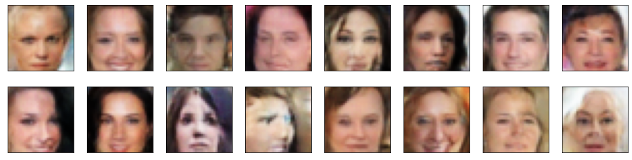
### Question: What do you notice about your generated samples and how might you improve this model?
When you answer this question, consider the following factors:
* The dataset is biased; it is made of "celebrity" faces that are mostly white
* Model size; larger models have the opportunity to learn more features in a data feature space
* Optimization strategy; optimizers and number of epochs affect your final result
**Answer:**
Initially, I ran this network for 10 epochs. I was able to generate face like objects (eyes, mouth, nose, hair) but the images were slightly disfigured. I then ran this network for 30 epochs, and achieved the results above. Here we can see clear human faces, with very little disfiguration or warping. One thing to notice, the sample output all appears to be female in nature. This might indicate a problem in the training.
As mentioned above, the data does seem to be biases as we have very little representation of black and asian races of both male and female. Also the training data does not have much in the way of glasses, hats and types of facial hair, religious headware, etc. My achieved results are quite indicitive of the data set itself. Lots of white generated faces.
Hiar color is another factor that has a pretty slim representation in the data. There are a few outliers that have hair that is not dark/blonde. Most of our generated faces have a hair color that falls into this region.
### Submitting This Project
When submitting this project, make sure to run all the cells before saving the notebook. Save the notebook file as "dlnd_face_generation.ipynb" and save it as a HTML file under "File" -> "Download as". Include the "problem_unittests.py" files in your submission.