https://github.com/d-krupke/cpsat-primer
The CP-SAT Primer: Using and Understanding Google OR-Tools' CP-SAT Solver
https://github.com/d-krupke/cpsat-primer
combinatorial-optimization cp-sat operations-research optimization ortools
Last synced: over 1 year ago
JSON representation
The CP-SAT Primer: Using and Understanding Google OR-Tools' CP-SAT Solver
- Host: GitHub
- URL: https://github.com/d-krupke/cpsat-primer
- Owner: d-krupke
- License: cc-by-4.0
- Created: 2022-07-10T08:00:40.000Z (about 4 years ago)
- Default Branch: main
- Last Pushed: 2024-10-24T19:01:13.000Z (over 1 year ago)
- Last Synced: 2024-10-30T03:42:41.468Z (over 1 year ago)
- Topics: combinatorial-optimization, cp-sat, operations-research, optimization, ortools
- Language: Jupyter Notebook
- Homepage: https://d-krupke.github.io/cpsat-primer/
- Size: 21.2 MB
- Stars: 367
- Watchers: 14
- Forks: 35
- Open Issues: 7
-
Metadata Files:
- Readme: README.md
- Contributing: CONTRIBUTING.md
- License: LICENSE
- Citation: CITATION.cff
Awesome Lists containing this project
- awesome_or-tools - CP-SAT Primer
README
*A book-style version of this primer is available at [https://d-krupke.github.io/cpsat-primer/](https://d-krupke.github.io/cpsat-primer/).*
# The CP-SAT Primer: Using and Understanding Google OR-Tools' CP-SAT Solver
_By [Dominik Krupke](https://krupke.cc), TU Braunschweig, with contributions
from Leon Lan, Michael Perk, and
[others](https://github.com/d-krupke/cpsat-primer/graphs/contributors)._
Many [combinatorially difficult](https://en.wikipedia.org/wiki/NP-hardness)
optimization problems can, despite their proven theoretical hardness, be solved
reasonably well in practice. The most successful approach is to use
[Mixed Integer Linear Programming](https://en.wikipedia.org/wiki/Integer_programming)
(MIP) to model the problem and then use a solver to find a solution. The most
successful solvers for MIPs are, e.g., [Gurobi](https://www.gurobi.com/),
[CPLEX](https://www.ibm.com/analytics/cplex-optimizer),
[COPT Cardinal Solver](https://www.copt.de/), and
[FICO Xpress Optimization](https://www.fico.com/en/products/fico-xpress-optimization),
which are all commercial and expensive (though, mostly free for academics).
There are also some open source solvers (e.g., [SCIP](https://www.scipopt.org/)
and [HiGHS](https://highs.dev/)), but they are often not as powerful as the
commercial ones (yet). However, even when investing in such a solver, the
underlying techniques
([Branch and Bound](https://en.wikipedia.org/wiki/Branch_and_bound) &
[Cut](https://en.wikipedia.org/wiki/Branch_and_cut) on
[Linear Relaxations](https://en.wikipedia.org/wiki/Linear_programming_relaxation))
struggle with some optimization problems, especially if the problem contains a
lot of logical constraints that a solution has to satisfy. In this case, the
[Constraint Programming](https://en.wikipedia.org/wiki/Constraint_programming)
(CP) approach may be more successful. For Constraint Programming, there are many
open source solvers, but they usually do not scale as well as MIP-solvers and
are worse in optimizing objective functions. While MIP-solvers are frequently
able to optimize problems with hundreds of thousands of variables and
constraints, the classical CP-solvers often struggle with problems with more
than a few thousand variables and constraints. However, the relatively new
[CP-SAT](https://developers.google.com/optimization/cp/cp_solver) of Google's
[OR-Tools](https://github.com/google/or-tools/) suite shows to overcome many of
the weaknesses and provides a viable alternative to MIP-solvers, being
competitive for many problems and sometimes even superior.
As a quick demonstration of CP-SAT's capabilities - particularly for those less
familiar with optimization frameworks - let us solve an instance of the NP-hard
Knapsack Problem. This classic optimization problem requires selecting a subset
of items, each with a specific weight and value, to maximize the total value
without exceeding a weight limit. Although a recursive algorithm is easy to
implement, 100 items yield approximately $2^{100} \approx 10^{30}$ possible
solutions. Even with a supercomputer performing $10^{18}$ operations per second,
it would take more than 31,000 years to evaluate all possibilities.
Here is how you can solve it using CP-SAT:
```python
from ortools.sat.python import cp_model # pip install -U ortools
# Specifying the input
weights = [395, 658, 113, 185, 336, 494, 294, 295, 256, 530, 311, 321, 602, 855, 209, 647, 520, 387, 743, 26, 54, 420, 667, 971, 171, 354, 962, 454, 589, 131, 342, 449, 648, 14, 201, 150, 602, 831, 941, 747, 444, 982, 732, 350, 683, 279, 667, 400, 441, 786, 309, 887, 189, 119, 209, 532, 461, 420, 14, 788, 691, 510, 961, 528, 538, 476, 49, 404, 761, 435, 729, 245, 204, 401, 347, 674, 75, 40, 882, 520, 692, 104, 512, 97, 713, 779, 224, 357, 193, 431, 442, 816, 920, 28, 143, 388, 23, 374, 905, 942]
values = [71, 15, 100, 37, 77, 28, 71, 30, 40, 22, 28, 39, 43, 61, 57, 100, 28, 47, 32, 66, 79, 70, 86, 86, 22, 57, 29, 38, 83, 73, 91, 54, 61, 63, 45, 30, 51, 5, 83, 18, 72, 89, 27, 66, 43, 64, 22, 23, 22, 72, 10, 29, 59, 45, 65, 38, 22, 68, 23, 13, 45, 34, 63, 34, 38, 30, 82, 33, 64, 100, 26, 50, 66, 40, 85, 71, 54, 25, 100, 74, 96, 62, 58, 21, 35, 36, 91, 7, 19, 32, 77, 70, 23, 43, 78, 98, 30, 12, 76, 38]
capacity = 2000
# Now we solve the problem
model = cp_model.CpModel()
xs = [model.new_bool_var(f"x_{i}") for i in range(len(weights))]
model.add(sum(x * w for x, w in zip(xs, weights)) <= capacity)
model.maximize(sum(x * v for x, v in zip(xs, values)))
solver = cp_model.CpSolver()
solver.solve(model)
print("Optimal selection:", [i for i, x in enumerate(xs) if solver.value(x)])
print("Total packed value:", solver.objective_value)
```
```
Optimal selection: [2, 14, 19, 20, 29, 33, 52, 53, 54, 58, 66, 72, 76, 77, 81, 86, 93, 94, 96]
Total packed value: 1161.0
```
How long did CP-SAT take? On my machine, it found the provably best solution
from $2^{100}$ possibilities in just 0.01 seconds. Feel free to try it on yours.
CP-SAT does not evaluate all solutions; it uses advanced techniques to make
deductions and prune the search space. While more efficient approaches than a
naive recursive algorithm exist, matching CP-SAT’s performance would require
significant time and effort. And this is just the beginning - CP-SAT can tackle
much more complex problems, as we will see in this primer.
> [!TIP]
>
> Not convinced yet of why tools like CP-SAT are amazing? Maybe Marco Lübbecke
> can convince you in his 12-minute TEDx talk
> [Anything you can do I can do better](https://www.youtube.com/watch?v=Dc38La-Xvog)
> about mathematical optimization.
### Content
Whether you are from the MIP community seeking alternatives or CP-SAT is your
first optimization solver, this book will guide you through the fundamentals of
CP-SAT in the first part, demonstrating all its features. The second part will
equip you with the skills needed to build and deploy optimization algorithms
using CP-SAT.
The first part introduces the fundamentals of CP-SAT, starting with a chapter on
installation. This chapter guides you through setting up CP-SAT and outlines the
necessary hardware requirements. The next chapter provides a simple example of
using CP-SAT, explaining the mathematical notation and its approximation in
Python with overloaded operators. You will then progress to basic modeling,
learning how to create variables, objectives, and fundamental constraints in
CP-SAT.
Following this, a chapter on advanced modeling will teach you how to handle
complex constraints, such as circuit constraints and intervals, with practical
examples. Another chapter discusses specifying CP-SAT's behavior, including
setting time limits and using parallelization. You will also find a chapter on
interpreting CP-SAT logs, which helps you understand how well CP-SAT is managing
your problem. Additionally, there is an overview of the underlying techniques
used in CP-SAT. The first part concludes with a chapter comparing CP-SAT with
other optimization techniques and tools, providing a broader context.
The second part delves into more advanced topics, focusing on general skills
like coding patterns and benchmarking rather than specific CP-SAT features. A
chapter on coding patterns offers basic design patterns for creating
maintainable algorithms with CP-SAT. Another chapter explains how to provide
your optimization algorithm as a service by building an optimization API. There
is also a chapter on developing powerful heuristics using CP-SAT for
particularly difficult or large problems. The second part concludes with a
chapter on benchmarking, offering guidance on how to scientifically benchmark
your model and interpret the results.
### Target Audience
I wrote this book for my computer science students at TU Braunschweig, and it is
used as supplementary material in my algorithm engineering courses. Initially,
we focused on Mixed Integer Programming (MIP), with CP-SAT discussed as an
alternative. However, we recently began using CP-SAT as the first optimization
solver due to its high-level interface, which is much easier for beginners to
grasp. Despite this shift, because MIP is more commonly used, the book includes
numerous comparisons to MIP. Thus, it is designed to be beginner-friendly while
also addressing the needs of MIP users seeking alternatives.
Unlike other books aimed at mathematical optimization or operations research
students, this one, aimed at computer science students, emphasizes coding over
mathematics or business cases, providing a hands-on approach to learning
optimization. The second part of the book can also be interesting for more
advanced users, providing content that I found missing in other books on
optimization.
### Table of Content
**Part 1: The Basics**
1. [Installation](#01-installation): Quick installation guide.
2. [Example](#02-example): A short example, showing the usage of CP-SAT.
3. [Basic Modeling](#04-modelling): An overview of variables, objectives, and
constraints.
4. [Advanced Modeling](#04B-advanced-modelling): More complex constraints, such
as circuit constraints and intervals.
5. [Parameters](#05-parameters): How to specify CP-SATs behavior, if needed.
Timelimits, hints, assumptions, parallelization, ...
6. [Understanding the Log](#understanding-the-log): How to interpret the log
7. [How does it work?](#07-under-the-hood): After we know what we can do with
CP-SAT, we look into how CP-SAT will do all these things.
8. [Alternatives](#03-big-picture): An overview of the different optimization
techniques and tools available. Putting CP-SAT into context.
**Part 2: Advanced Topics**
7. [Coding Patterns](#06-coding-patterns): Basic design patterns for creating
maintainable algorithms.
8. [(DRAFT) Building an Optimization API](#building_an_optimization_api) How to
build a scalable API for long running optimization jobs.
9. [(DRAFT) CP-SAT vs. ML vs. QC](#chapters-machine-learning): A comparison of
CP-SAT with Machine Learning and Quantum Computing.
10. [Large Neighborhood Search](#09-lns): The use of CP-SAT to create more
powerful heuristics.
11. [Benchmarking your Model](#08-benchmarking): How to benchmark your model and
how to interpret the results.
### Background
This book assumes you are fluent in Python, and have already been introduced to
combinatorial optimization problems. In case you are just getting into
combinatorial optimization and are learning on your own, I recommend starting
with the free Coursera course,
[Discrete Optimization](https://www.coursera.org/learn/discrete-optimization),
taught by Pascal Van Hentenryck and Carleton Coffrin. This course provides a
comprehensive introduction in a concise format.
For an engaging exploration of a classic problem within this domain,
[In Pursuit of the Traveling Salesman by Bill Cook](https://press.princeton.edu/books/paperback/9780691163529/in-pursuit-of-the-traveling-salesman)
is highly recommended. This book, along with this
[YouTube talk](https://www.youtube.com/watch?v=5VjphFYQKj8) by the author that
lasts about an hour, offers a practical case study of the well-known Traveling
Salesman Problem. It not only introduces fundamental techniques but also delves
into the community and historical context of the field.
Additionally, the article
[Mathematical Programming](https://www.gurobi.com/resources/math-programming-modeling-basics/)
by CP-SAT's competitor Gurobi offers an insightful introduction to mathematical
programming and modeling. In this context, the term "Programming" does not refer
to coding; rather, it originates from an earlier usage of the word "program",
which denoted a plan of action or a schedule. If this distinction is new to you,
it is a strong indication that you would benefit from reading this article.
> **About the Lead Author:** [Dr. Dominik Krupke](https://krupke.cc) is a
> postdoctoral researcher with the
> [Algorithms Division](https://www.ibr.cs.tu-bs.de/alg) at TU Braunschweig. He
> specializes in practical solutions to NP-hard problems. Initially focused on
> theoretical computer science, he now applies his expertise to solve what was
> once deemed impossible, frequently with the help of CP-SAT. This primer on
> CP-SAT, first developed as course material for his students, has been extended
> in his spare time to cater to a wider audience.
>
> **Contributors:** This primer has been enriched by the contributions of
> [several individuals](https://github.com/d-krupke/cpsat-primer/graphs/contributors).
> Notably, Leon Lan played a key role in restructuring the content and offering
> critical feedback, while Michael Perk significantly enhanced the section on
> the reservoir constraint. I also extend my gratitude to all other contributors
> who identified and corrected errors, improved the text, and offered valuable
> insights.
> **Found a mistake?** Please open an issue or a pull request. You can also just
> write me a quick mail to `krupked@gmail.com`.
> **Want to contribute?** If you are interested in contributing, please open an
> issue or email me with a brief description of your proposal. We can then
> discuss the details. I welcome all assistance and am open to expanding the
> content. Contributors to any section or similar input will be recognized as
> coauthors.
> **Want to use/share this content?** This tutorial can be freely used under
> [CC-BY 4.0](https://creativecommons.org/licenses/by/4.0/). Smaller parts can
> even be copied without any acknowledgement for non-commercial, educational
> purposes.
---
# Part 1: The Basics
## Installation
We are using Python 3 in this primer and assume that you have a working Python 3
installation as well as the basic knowledge to use it. There are also interfaces
for other languages, but Python 3 is, in my opinion, the most convenient one, as
the mathematical expressions in Python are very close to the mathematical
notation (allowing you to spot mathematical errors much faster). Only for huge
models, you may need to use a compiled language such as C++ due to performance
issues. For smaller models, you will not notice any performance difference.
The installation of CP-SAT, which is part of the OR-Tools package, is very easy
and can be done via Python's package manager
[pip](https://pip.pypa.io/en/stable/).
```shell
pip3 install -U ortools
```
This command will also update an existing installation of OR-Tools. As this tool
is in active development, it is recommended to update it frequently. We actually
encountered wrong behavior, i.e., bugs, in earlier versions that then have been
fixed by updates (this was on some more advanced features, do not worry about
correctness with basic usage).
I personally like to use [Jupyter Notebooks](https://jupyter.org/) for
experimenting with CP-SAT.
### What hardware do you need?
It is important to note that for CP-SAT usage, you do not need the capabilities
of a supercomputer. A standard laptop is often sufficient for solving many
problems. The primary requirements are CPU power and memory bandwidth, with a
GPU being unnecessary.
In terms of CPU power, the key is balancing the number of cores with the
performance of each individual core. CP-SAT leverages all available cores by
default, implementing different strategies on each.
[Depending on the number of cores, CP-SAT will behave differently](https://github.com/google/or-tools/blob/main/ortools/sat/docs/troubleshooting.md#improving-performance-with-multiple-workers).
However, the effectiveness of these strategies can vary, and it is usually not
apparent which one will be most effective. A higher single-core performance
means that your primary strategy will operate more swiftly. I recommend a
minimum of 4 cores and 16GB of RAM.
While CP-SAT is quite efficient in terms of memory usage, the amount of
available memory can still be a limiting factor in the size of problems you can
tackle. When it came to setting up our lab for extensive benchmarking at TU
Braunschweig, we faced a choice between desktop machines and more expensive
workstations or servers. We chose desktop machines equipped with AMD Ryzen 9
7900 CPUs (Intel would be equally suitable) and 96GB of DDR5 RAM, managed using
Slurm. This decision was driven by the fact that the performance gains from
higher-priced workstations or servers were relatively marginal compared to their
significantly higher costs. When on the road, I am often still able to do stuff
with my old Intel Macbook Pro from 2018 with an i7 and only 16GB of RAM, but
large models will overwhelm it. My workstation at home with AMD Ryzen 7 5700X
and 32GB of RAM on the other hand rarely has any problems with the models I am
working on.
For further guidance, consider the
[hardware recommendations for the Gurobi solver](https://support.gurobi.com/hc/en-us/articles/8172407217041-What-hardware-should-I-select-when-running-Gurobi-),
which are likely to be similar. Since we frequently use Gurobi in addition to
CP-SAT, our hardware choices were also influenced by their recommendations.
## A Simple Example
Before we dive into any internals, let us take a quick look at a simple
application of CP-SAT. This example is so simple that you could solve it by
hand, but know that CP-SAT would (probably) be fine with you adding a thousand
(maybe even ten- or hundred-thousand) variables and constraints more. The basic
idea of using CP-SAT is, analogous to MIPs, to define an optimization problem in
terms of variables, constraints, and objective function, and then let the solver
find a solution for it. We call such a formulation that can be understood by the
corresponding solver a _model_ for the problem. For people not familiar with
this
[declarative approach](https://programiz.pro/resources/imperative-vs-declarative-programming/),
you can compare it to SQL, where you also just state what data you want, not how
to get it. However, it is not purely declarative, because it can still make a
huge(!) difference how you model the problem and getting that right takes some
experience and understanding of the internals. You can still get lucky for
smaller problems (let us say a few hundred to thousands of variables) and obtain
optimal solutions without having an idea of what is going on. The solvers can
handle more and more 'bad' problem models effectively with every year.
> [!NOTE]
>
> A **model** in mathematical programming refers to a mathematical description
> of a problem, consisting of variables, constraints, and optionally an
> objective function that can be understood by the corresponding solver class.
> _Modelling_ refers to transforming a problem (instance) into the corresponding
> framework, e.g., by making all constraints linear as required for Mixed
> Integer Linear Programming. Be aware that the
> [SAT](https://en.wikipedia.org/wiki/SAT_solver)-community uses the term
> _model_ to refer to a (feasible) variable assignment, i.e., solution of a
> SAT-formula. If you struggle with this terminology, maybe you want to read
> this short guide on
> [Math Programming Modelling Basics](https://www.gurobi.com/resources/math-programming-modeling-basics/).
Our first problem has no deeper meaning, except for showing the basic workflow
of creating the variables (x and y), adding the constraint $x+y<=30$ on them,
setting the objective function (maximize $30x + 50y$), and obtaining a solution:
```python
from ortools.sat.python import cp_model
model = cp_model.CpModel()
# Variables
x = model.new_int_var(0, 100, "x")
y = model.new_int_var(0, 100, "y")
# Constraints
model.add(x + y <= 30)
# Objective
model.maximize(30 * x + 50 * y)
# Solve
solver = cp_model.CpSolver()
status_code = solver.solve(model)
status_name = solver.status_name()
# Print the solver status and the optimal solution.
print(f"{status_name} ({status_code})")
print(f"x={solver.value(x)}, y={solver.value(y)}")
```
OPTIMAL (4)
x=0, y=30
Pretty easy, right? For solving a generic problem, not just one specific
instance, you would of course create a dictionary or list of variables and use
something like `model.add(sum(vars)<=n)`, because you do not want to create the
model by hand for larger instances.
> [!TIP]
>
> The solver can return five different statuses:
>
> | Status | Code | Description |
> | --------------- | ---- | ------------------------------------------------------------------------------------------------------------------------------------------------------------------------------------- |
> | `UNKNOWN` | 0 | The solver has not run for long enough. |
> | `MODEL_INVALID` | 1 | The model is invalid. You will rarely see that status. |
> | `FEASIBLE` | 2 | The model has a feasible, but not necessarily optimal, solution. If your model does not have an objective, every feasible model will return `OPTIMAL`, which may be counterintuitive. |
> | `INFEASIBLE` | 3 | The model has no feasible solution. This means that your constraints are too restrictive. |
> | `OPTIMAL` | 4 | The model has an optimal solution. If your model does not have an objective, `OPTIMAL` is returned instead of `FEASIBLE`. |
>
> The status `UNBOUNDED` does _not_ exist, as CP-SAT does not have unbounded
> variables.
For larger models, CP-SAT will unfortunately not always able to compute an
optimal solution. However, the good news is that the solver will likely still
find a satisfactory solution and provide a bound on the optimal solution. Once
you reach this point, understanding how to interpret the solver's log becomes
crucial for analyzing the solver's performance. We will learn more about this
later.
### Mathematical Model
The mathematical model of the code above would usually be written by experts
something like this:
```math
\max 30x + 50y
```
```math
\text{s.t. } x+y \leq 30
```
```math
\quad 0\leq x \leq 100
```
```math
\quad 0\leq y \leq 100
```
```math
x,y \in \mathbb{Z}
```
The `s.t.` stands for `subject to`, sometimes also read as `such that`.
### Overloading
One aspect of using CP-SAT solver that often poses challenges for learners is
understanding operator overloading in Python and the distinction between the two
types of variables involved. In this context, `x` and `y` serve as mathematical
variables. That is, they are placeholders that will only be assigned specific
values during the solving phase. To illustrate this more clearly, let us explore
an example within the Python shell:
```pycon
>>> model = cp_model.CpModel()
>>> x = model.new_int_var(0, 100, "x")
>>> x
x(0..100)
>>> type(x)
>>> x + 1
sum(x(0..100), 1)
>>> x + 1 <= 1
```
In this example, `x` is not a conventional number but a placeholder defined to
potentially assume any value between 0 and 100. When 1 is added to `x`, the
result is a new placeholder representing the sum of `x` and 1. Similarly,
comparing this sum to 1 produces another placeholder, which encapsulates the
comparison of the sum with 1. These placeholders do not hold concrete values at
this stage but are essential for defining constraints within the model.
Attempting operations like `if x + 1 <= 1: print("True")` will trigger a
`NotImplementedError`, as the condition `x+1<=1` cannot be evaluated directly.
Although this approach to defining models might initially seem perplexing, it
facilitates a closer alignment with mathematical notation, which in turn can
make it easier to identify and correct errors in the modeling process.
### More examples
If you are not yet satisfied,
[this folder contains many Jupyter Notebooks with examples from the developers](https://github.com/google/or-tools/tree/stable/examples/notebook/sat).
For example
- [multiple_knapsack_sat.ipynb](https://github.com/google/or-tools/blob/stable/examples/notebook/sat/multiple_knapsack_sat.ipynb)
shows how to solve a multiple knapsack problem.
- [nurses_sat.ipynb](https://github.com/google/or-tools/blob/stable/examples/notebook/sat/nurses_sat.ipynb)
shows how to schedule the shifts of nurses.
- [bin_packing_sat.ipynb](https://github.com/google/or-tools/blob/stable/examples/notebook/sat/bin_packing_sat.ipynb)
shows how to solve a bin packing problem.
- ... (if you know more good examples I should mention here, please let me
know!)
Further, you can find an extensive and beginner-friendly example on scheduling
workers
[here](https://pganalyze.com/blog/a-practical-introduction-to-constraint-programming-using-cp-sat).
Now that you have seen a minimal model, let us explore the various options
available for problem modeling. While an experienced optimizer might be able to
handle most problems using just the elements previously discussed, clearly
expressing your intentions can help CP-SAT optimize your problem more
effectively.
---
## Basic Modeling
In this chapter, we dive into the basic modeling capabilities of CP-SAT. CP-SAT
provides an extensive set of constraints, closer to high-level modeling
languages like MiniZinc than to traditional Mixed Integer Programming (MIP). For
example, it offers constraints like `all_different` and
`add_multiplication_equality`. These advanced features reduce the need for
modeling complex logic strictly through linear constraints, though they also
increase the interface's complexity. However, not all constraints are equally
efficient; linear and boolean constraints are generally most efficient, whereas
constraints like `add_multiplication_equality` can be significantly more
resource-intensive.
> [!TIP]
>
> If you are transitioning from Mixed Integer Programming (MIP), you might be
> used to manually implementing higher-level constraints and optimizing Big-M
> parameters for better performance. With CP-SAT, such manual adjustments are
> generally unnecessary. CP-SAT operates differently from typical MIP solvers by
> relying less on linear relaxation and more on its underlying SAT-solver and
> propagators to efficiently manage logical constraints. Embrace the
> higher-level constraints—they are often more efficient in CP-SAT.
This primer has been expanded to cover all constraints across two chapters,
complete with various examples to illustrate the contexts in which they can be
used. However, mastering modeling involves much more than just an understanding
of constraints. It requires a deep appreciation of the principles and techniques
that make models effective and applicable to real-world problems.
For a more detailed exploration of modeling, consider "Model Building in
Mathematical Programming" by H. Paul Williams, which offers extensive insight
into the subject, including practical applications. While this book is not
specific to CP-SAT, the foundational techniques and concepts are broadly
applicable. Additionally, for those new to this area or transitioning from MIP
solutions, studying Gurobi's modeling approach through this
[video course](https://www.youtube.com/playlist?list=PLHiHZENG6W8CezJLx_cw9mNqpmviq3lO9)
might prove helpful. While many principles overlap, some strategies unique to
CP-SAT can better address cases where traditional MIP-solvers struggle.
Additional resources on mathematical modeling (not CP-SAT specific):
- [Math Programming Modeling Basics by Gurobi](https://www.gurobi.com/resources/math-programming-modeling-basics/):
This resource provides a solid introduction to the basics of mathematical
modeling.
- [Modeling with Gurobi Python](https://www.youtube.com/playlist?list=PLHiHZENG6W8CezJLx_cw9mNqpmviq3lO9):
A comprehensive video course on modeling with Gurobi, highlighting concepts
that are also applicable to CP-SAT.
- [Model Building in Mathematical Programming by H. Paul Williams](https://www.wiley.com/en-us/Model+Building+in+Mathematical+Programming%2C+5th+Edition-p-9781118443330):
An extensive guide to mathematical modeling techniques.
> [!TIP]
>
> For getting started with implementing optimization models in general, I highly
> recommend the blog post
> [The Art Of Not Making It An Art](https://www.gurobi.com/resources/optimization-modeling-the-art-of-not-making-it-an-art/).
> It excellently summarizes the fundamental principles of successfully managing
> an optimization project, independent of the concrete language or solver.
---
**Elements:**
- [Variables](#04-modelling-variables): `new_int_var`, `new_bool_var`,
`new_constant`, `new_int_var_series`, `new_bool_var_series`
- [Custom Domain Variables](#04-modelling-domain-variables):
`new_int_var_from_domain`
- [Objectives](#04-modelling-objectives): `minimize`, `maximize`
- [Linear Constraints](#04-modelling-linear-constraints): `add`,
`add_linear_constraint`
- [Logical Constraints (Propositional Logic)](#04-modelling-logic-constraints):
`add_implication`, `add_bool_or`, `add_at_least_one`, `add_at_most_one`,
`add_exactly_one`, `add_bool_and`, `add_bool_xor`
- [Conditional Constraints (Reification)](#04-modelling-conditional-constraints):
`only_enforce_if`
- [Absolute Values and Max/Min](#04-modelling-absmaxmin): `add_min_equality`,
`add_max_equality`, `add_abs_equality`
- [Multiplication, Division, and Modulo](#04-modelling-multdivmod):
`add_modulo_equality`, `add_multiplication_equality`, `add_division_equality`
- [All Different](#04-modelling-alldifferent): `add_all_different`
- [Domains and Combinations](#04-modelling-table): `add_allowed_assignments`,
`add_forbidden_assignments`
- [Array/Element Constraints](#04-modelling-element): `add_element`,
`add_inverse`
The more advanced constraints `add_circuit`, `add_multiple_circuit`,
`add_automaton`,`add_reservoir_constraint`,
`add_reservoir_constraint_with_active`, `new_interval_var`,
`new_interval_var_series`, `new_fixed_size_interval_var`,
`new_optional_interval_var`, `new_optional_interval_var_series`,
`new_optional_fixed_size_interval_var`,
`new_optional_fixed_size_interval_var_series`, `add_no_overlap`,
`add_no_overlap_2d`, and `add_cumulative` are discussed in the next chapter.
---
### Variables
There are two important types of variables in CP-SAT: Booleans and Integers
(which are actually converted to Booleans, but more on this later). There are
also, e.g.,
[interval variables](https://developers.google.com/optimization/reference/python/sat/python/cp_model#intervalvar),
but they are actually rather a combination of integral variables and discussed
[later](#04-modelling-intervals). For the integer variables, you have to specify
a lower and an upper bound.
```python
model = cp_model.CpModel()
# Integer variable z with bounds -100 <= z <= 100
z = model.new_int_var(-100, 100, "z") # new syntax
z_ = model.NewIntVar(-100, 100, "z_") # old syntax
# Boolean variable b
b = model.new_bool_var("b") # new syntax
b_ = model.NewBoolVar("b_") # old syntax
# Implicitly available negation of b:
not_b = ~b # will be 1 if b is 0 and 0 if b is 1
not_b_ = b.Not() # old syntax
```
Additionally, you can use `model.new_int_var_series` and
`model.new_bool_var_series` to create multiple variables at once from a pandas
Index. This is especially useful if your data is given in a pandas DataFrame.
However, there is no performance benefit in using this method, it is just more
convenient.
```python
model = cp_model.CpModel()
# Create an Index from 0 to 9
index = pd.Index(range(10), name="index")
# Create a pandas Series with 10 integer variables matching the index
xs = model.new_int_var_series("x", index, 0, 100)
# List of boolean variables
df = pd.DataFrame(
data={"weight": [1 for _ in range(10)], "value": [3 for _ in range(10)]},
index=["A", "B", "C", "D", "E", "F", "G", "H", "I", "J"],
)
bs = model.new_bool_var_series("b", df.index) # noqa: F841
# Using the dot product on the pandas DataFrame is actually a pretty
# convenient way to create common linear expressions.
model.add(bs @ df["weight"] <= 100)
model.maximize(bs @ df["value"])
```
Additionally, there is the `new_constant`-method, which allows you to create a
variable that is constant. This allows you to safely replace variables by
constants. This is primarily useful for boolean variables, as constant integer
variables can in most cases be simply replaced by plain integers.
> [!TIP]
>
> In an older project, I observed that maintaining tight bounds on integer
> variables can significantly impact performance. Employing a heuristic to find
> a reasonable initial solution, which then allowed for tighter bounds, proved
> worthwhile, even though the bounds were just a few percent tighter. Although
> this project was several years ago and CP-SAT has advanced considerably since
> then, I still recommend keeping the bounds on the variables' ranges as tight
> as possible.
There are no continuous/floating point variables (or even constants) in CP-SAT:
If you need floating point numbers, you have to approximate them with integers
by some resolution. For example, you could simply multiply all values by 100 for
a step size of 0.01. A value of 2.35 would then be represented by 235. This
_could_ probably be implemented in CP-SAT directly, but doing it explicitly is
not difficult, and it has numerical implications that you should be aware of.
The absence of continuous variables may appear as a substantial limitation,
especially for those with a background in linear optimization where continuous
variables are typically regarded as the simpler component. However, if your
problem includes only a few continuous variables that must be approximated using
large integers and involves complex constraints such as absolute values, while
the majority of the problem is dominated by logical constraints, CP-SAT can
often outperform mixed-integer programming solvers. It is only when a problem
contains a substantial number of continuous variables and benefits significantly
from strong linear relaxation that mixed-integer programming solvers will have a
distinct advantage, despite CP-SAT having a propagator based on the dual simplex
method.
I analyzed the impact of resolution (i.e., the factor by which floating point
numbers are multiplied) on the runtime of CP-SAT, finding that the effect varied
depending on the problem. For one problem, the runtime increased only
logarithmically with the resolution, allowing the use of a very high resolution
of 100,000x without significant issues. In contrast, for another problem, the
runtime increased roughly linearly with the resolution, making high resolutions
impractical. The runtime for different factors in this case was: 1x: 0.02s, 10x:
0.7s, 100x: 7.6s, 1000x: 75s, and 10,000x: over 15 minutes, even though the
solution remained the same, merely scaled. Therefore, while high resolutions may
be feasible for some problems using CP-SAT, it is essential to verify their
influence on runtime, as the impact can be considerable.
In my experience, boolean variables are crucial in many combinatorial
optimization problems. For instance, the famous Traveling Salesman Problem
consists solely of boolean variables. Therefore, implementing a solver that
specializes in boolean variables using a SAT-solver as a foundation, such as
CP-SAT, is a sensible approach. CP-SAT leverages the strengths of SAT-solving
techniques, which are highly effective for problems dominated by boolean
variables.
You may wonder why it is necessary to explicitly name the variables in CP-SAT.
While there does not appear to be a technical reason for this requirement,
naming the variables can be extremely helpful for debugging purposes.
Understanding the naming scheme of the variables allows you to more easily
interpret the internal representation of the model, facilitating the
identification and resolution of issues. To be fair, there have only been a few
times when I actually needed to take a closer at the internal representation,
and in most of the cases I would have preferred not to have to name the
variables.
#### Custom Domain Variables
When dealing with integer variables that you know will only need to take certain
values, or when you wish to limit their possible values, custom domain variables
can become interesting. Unlike regular integer variables, which must have a
domain between a given range of values (e.g., $\[ 1, 100 \]$), domain variables
can specify a custom set of values as domain (e.g., $\\{1, 3, 5 \\}$). This
approach can enhance efficiency when the domain - the range of sensible values -
is small. However, it may not be the best choice for larger domains.
CP-SAT works by converting all integer variables into boolean variables
(warning: simplification). For each potential value, it creates two boolean
variables: one indicating whether the integer variable is equal to this value,
and another indicating whether it is less than or equal to it. This is called an
_order encoding_. At first glance, this might suggest that using domain
variables is always preferable, as it appears to reduce the number of boolean
variables needed.
However, CP-SAT employs a lazy creation strategy for these boolean variables.
This means it only generates them as needed, based on the solver's
decision-making process. Therefore, an integer variable with a wide range - say,
from 0 to 100 - will not immediately result in 200 boolean variables. It might
lead to the creation of only a few, depending on the solver's requirements.
Limiting the domain of a variable can have drawbacks. Firstly, defining a domain
explicitly can be computationally costly and increase the model size drastically
as it now need to contain not just a lower and upper bound for a variable but an
explicit list of numbers (model size is often a limiting factor). Secondly, by
narrowing down the solution space, you might inadvertently make it more
challenging for the solver to find a viable solution. First, try to let CP-SAT
handle the domain of your variables itself and only intervene if you have a good
reason to do so.
If you choose to utilize domain variables for their benefits in specific
scenarios, here is how to define them:
```python
from ortools.sat.python import cp_model
model = cp_model.CpModel()
# Define a domain with selected values
domain = cp_model.Domain.from_values([2, 5, 8, 10, 20, 50, 90])
# Can also be done via intervals
domain_2 = cp_model.Domain.from_intervals([[8, 12], [14, 20]])
# There are also some operations available
domain_3 = domain.union_with(domain_2)
# Create a domain variable within this defined domain
x = model.new_int_var_from_domain(domain, "x")
```
This example illustrates the process of creating a domain variable `x` that can
only take on the values specified in `domain`. This method is particularly
useful when you are working with variables that only have a meaningful range of
possible values within your problem's context.
### Objectives
Not every problem necessitates an objective; sometimes, finding a feasible
solution is sufficient. CP-SAT excels at finding feasible solutions, a task at
which mixed-integer programming (MIP) solvers often do not perform as well.
However, CP-SAT is also capable of effective optimization, which is an area
where older constraint programming solvers may lag, based on my experience.
CP-SAT allows for the minimization or maximization of a linear expression. You
can model more complex expressions by using auxiliary variables and additional
constraints. To specify an objective function, you can use the `model.minimize`
or `model.maximize` commands with a linear expression. This flexibility makes
CP-SAT a robust tool for a variety of optimization tasks.
```python
# Basic model with variables and constraints
model = cp_model.CpModel()
x = model.new_int_var(-100, 100, "x")
y = model.new_int_var(-100, 100, "y")
model.add(x + 10 * y <= 100)
# Minimize 30x + 50y
model.maximize(30 * x + 50 * y)
```
Let us look on how to model more complicated expressions, using boolean
variables and generators.
```python
model = cp_model.CpModel()
x_vars = [model.new_bool_var(f"x{i}") for i in range(10)]
model.minimize(sum(i * x_vars[i] if i % 2 == 0 else i * ~x_vars[i] for i in range(10)))
```
This objective evaluates to
```math
\min \sum_{i=0}^{9} i\cdot x_i \text{ if } i \text{ is even else } i\cdot \neg x_i
```
To implement a
[lexicographic optimization](https://en.wikipedia.org/wiki/Lexicographic_optimization),
you can do multiple rounds and always fix the previous objective as constraint.
```python
# some basic model
model = cp_model.CpModel()
x = model.new_int_var(-100, 100, "x")
y = model.new_int_var(-100, 100, "y")
z = model.new_int_var(-100, 100, "z")
model.add(x + 10 * y - 2 * z <= 100)
# Define the objectives
first_objective = 30 * x + 50 * y
second_objective = 10 * x + 20 * y + 30 * z
# Optimize for the first objective
model.maximize(first_objective)
solver = cp_model.CpSolver()
solver.solve(model)
# Fix the first objective and optimize for the second
model.add(first_objective == int(solver.objective_value)) # fix previous objective
model.minimize(second_objective) # optimize for second objective
solver.solve(model)
```
> [!TIP]
>
> You can find a more efficient implementation of lexicographic optimization in
> the _Coding Patterns_ chapter.
To handle non-linear objectives in CP-SAT, you can employ auxiliary variables
and constraints. For instance, to incorporate the absolute value of a variable
into your objective, you first create a new variable representing this absolute
value. Shortly, you will learn more about setting up these types of constraints.
Below is a Python example demonstrating how to model and minimize the absolute
value of a variable `x`:
```python
# Assuming x is already defined in your model
abs_x = model.new_int_var(
0, 100, "|x|"
) # Create a variable to represent the absolute value of x
model.add_abs_equality(target=abs_x, expr=x) # Define abs_x as the absolute value of x
model.minimize(abs_x) # Set the objective to minimize abs_x
```
The constraints available to define your feasible solution space will be
discussed in the following section.
### Linear Constraints
These are the classical constraints also used in linear optimization. Remember
that you are still not allowed to use floating point numbers within it. Same as
for linear optimization: You are not allowed to multiply a variable with
anything else than a constant and also not to apply any further mathematical
operations.
```python
model.add(10 * x + 15 * y <= 10)
model.add(x + z == 2 * y)
# This one actually is not linear but still works.
model.add(x + y != z)
# Because we are working on integers, the true smaller or greater constraints
# are trivial to implement as x < z is equivalent to x <= z-1
model.add(x < y + z)
model.add(y > 300 - 4 * z)
```
Note that `!=` can be slower than the other (`<=`, `>=`, `==`) constraints,
because it is not a linear constraint. If you have a set of mutually `!=`
variables, it is better to use `all_different` (see below) than to use the
explicit `!=` constraints.
> [!WARNING]
>
> If you use intersecting linear constraints, you may get problems because the
> intersection point needs to be integral. There is no such thing as a
> feasibility tolerance as in Mixed Integer Programming-solvers, where small
> deviations are allowed. The feasibility tolerance in MIP-solvers allows, e.g.,
> 0.763445 == 0.763439 to still be considered equal to counter numerical issues
> of floating point arithmetic. In CP-SAT, you have to make sure that values can
> match exactly.
Let us look at the following example with two linear equality constraints:
```math
x - y = 0
```
```math
4-y = 2y
```
```math
x, y \geq 0
```
You can verify that $x=4/3$ and $y=4/3$ is a feasible solution. However, coding
this in CP-SAT results in an infeasible solution:
```python
model = cp_model.CpModel()
x = model.new_int_var(-100, 100, "x")
y = model.new_int_var(-100, 100, "y")
model.add(x - y == 0)
model.add(4 - x == 2 * y)
solver = cp_model.CpSolver()
status = solver.solve(model)
assert status == cp_model.INFEASIBLE
```
Even using scaling techniques, such as multiplying integer variables by
1,000,000 to increase the resolution, would not render the model feasible. While
common linear programming solvers would handle this model without issue, CP-SAT
struggles unless modifications are made to eliminate fractions, such as
multiplying all terms by 3. However, this requires manual intervention, which
undermines the idea of using a solver. These limitations are important to
consider, although such scenarios are rare in practical applications.
> [!TIP]
>
> If you have long sums of variables and coefficients, it can be more efficient
> to use the sum-methods of LinearExpr than to use Python's sum-function. Note
> that this function does currently not support generators.
>
> ```python
> xs = [model.NewIntVar(0, 10, f"x{i}") for i in range(5)]
> weights = [i for i in range(5)]
> model.add(cp_model.LinearExpr.sum(xs) >= 1)
> model.minimize(cp_model.LinearExpr.weighted_sum(xs, weights))
> ```
If you have a lower and an upper bound for a linear expression, you can also use
the `add_linear_constraint`-method, which allows you to specify both bounds in
one go.
```python
model.add_linear_constraint(linear_expr=10 * x + 15 * y, lb=-100, ub=10)
```
The similar sounding `AddLinearExpressionInDomain` is discussed later.
### Logical Constraints (Propositional Logic)
Propositional logic allows us to describe relationships between true or false
statements using logical operators. Consider a simple scenario where we define
three Boolean variables:
```python
b1 = model.new_bool_var("b1")
b2 = model.new_bool_var("b2")
b3 = model.new_bool_var("b3")
```
These variables, `b1`, `b2`, and `b3`, represent distinct propositions whose
truth values are to be determined by the model.
You can obtain the negation of a Boolean variable by using `~` or the
`.Not()`-method. The resulting variable can be used just like the original
variable:
```python
not_b1 = ~b1 # Negation of b1
not_b2 = b2.Not() # Alternative notation for negation
```
Note that you can use more than three variables in all of the following
examples, except for `add_implication` which is only defined for two variables.
> [!WARNING]
>
> Boolean variables are essentially special integer variables restricted to the
> domain of 0 and 1. Therefore, you can incorporate them into linear constraints
> as well. However, it is important to note that integer variables, unlike
> Boolean variables, cannot be used in Boolean constraints. This is a
> distinction from some programming languages, like Python, where integers can
> sometimes substitute for Booleans.
#### Adding Logical OR Constraints
The logical OR operation ensures that at least one of the specified conditions
holds true. To model this, you can use:
```python
model.add_bool_or(b1, b2, b3) # b1 or b2 or b3 must be true
model.add_at_least_one([b1, b2, b3]) # Alternative notation
model.add(b1 + b2 + b3 >= 1) # Alternative linear notation using '+' for OR
```
Both lines ensure that at least one of `b1`, `b2`, or `b3` is true.
#### Adding Logical AND Constraints
The logical AND operation specifies that all conditions must be true
simultaneously. To model conditions where `b1` is true and both `b2` and `b3`
are false, you can use:
```python
model.add_bool_and(b1, b2.Not(), b3.Not()) # b1 and not b2 and not b3 must all be true
model.add_bool_and(b1, ~b2, ~b3) # Alternative notation using '~' for negation
```
The `add_bool_and` method is most effective when used with the `only_enforce_if`
method (discussed in
[Conditional Constraints (Reification)](#04-modelling-conditional-constraints)).
For cases not utilizing `only_enforce_if` a simple AND-clause such as
$\left( b_1 \land \neg b_2 \land \neg b_3 \right)$ becomes redundant by simply
substituting $b_1$ with `1` and $b_2, b_3$ with `0`. In straightforward
scenarios, consider substituting these variables with their constant values to
reduce unnecessary complexity, especially in larger models where size and
manageability are concerns. In smaller or simpler models, CP-SAT efficiently
handles these redundancies, allowing you to focus on maintaining clarity and
readability in your model.
#### Adding Logical XOR Constraints
The logical XOR (exclusive OR) operation ensures that an odd number of operands
are true. It is crucial to understand this definition, as it has specific
implications when applied to more than two variables:
- For two variables, such as `b1 XOR b2`, the operation returns true if exactly
one of these variables is true, which aligns with the "exactly one" constraint
for this specific case.
- For three or more variables, such as in the expression `b1 XOR b2 XOR b3`, the
operation returns true if an odd number of these variables are true. This
includes scenarios where one or three variables are true, assuming the total
number of variables involved is three.
This characteristic of XOR can be somewhat complex but is crucial for modeling
scenarios where the number of true conditions needs to be odd:
```python
model.add_bool_xor(b1, b2) # Returns true if exactly one of b1 or b2 is true
model.add_bool_xor(
b1, b2, b3
) # Returns true if an odd number of b1, b2, b3 are true (i.e., one or three)
```
#### Specifying Unique Conditions
To enforce that exactly one or at most one of the variables is true, use:
```python
model.add_exactly_one([b1, b2, b3]) # Exactly one of the variables must be true
model.add_at_most_one([b1, b2, b3]) # No more than one of the variables should be true
```
These constraints are useful for scenarios where exclusive choices must be
modeled.
You could alternatively also use `add`.
```python
model.add(b1 + b2 + b3 == 1) # Exactly one of the variables must be true
model.add(b1 + b2 + b3 <= 1) # No more than one of the variables should be true
```
#### Modeling Implications
Logical implication, denoted as `->`, indicates that if the first condition is
true, the second must also be true. This can be modeled as:
```python
model.add_implication(b1, b2) # If b1 is true, then b2 must also be true
```
You could also use `add`.
```python
model.add(b2 >= b1) # If b1 is true, then b2 must also be true
```
### Conditional Constraints (Reification)
In practical applications, scenarios often arise where conditions dictate the
enforcement of certain constraints. For instance, "if this condition is true,
then a specific constraint should apply," or "if a constraint is violated, a
penalty variable is set to true, triggering another constraint." Additionally,
real-world constraints can sometimes be bypassed with financial or other types
of concessions, such as renting a more expensive truck to exceed a load limit,
or allowing a worker to take a day off after a double shift.
> In constraint programming, **reification** involves associating a Boolean
> variable with a constraint to capture its truth value, thereby turning the
> satisfaction of the constraint into a variable that can be used in further
> constraints. Full reification links a Boolean variable such that it is `True`
> if the constraint is satisfied and `False` otherwise, enabling the variable to
> be directly used in other decisions or constraints. Conversely,
> half-reification, or implied constraints, involves a one-way linkage where the
> Boolean variable being `True` implies the constraint must be satisfied, but
> its being `False` does not necessarily indicate anything about the
> constraint's satisfaction. This approach is particularly useful for expressing
> complex conditional logic and for modeling scenarios where only the
> satisfaction, and not the violation, of a constraint needs to be explicitly
> handled.
To effectively manage these conditional scenarios, CP-SAT offers the
`only_enforce_if`-method for linear and some Boolean constraints, which
activates a constraint only if a specified condition is met. This method is not
only typically more efficient than traditional methods like the
[Big-M method](https://en.wikipedia.org/wiki/Big_M_method) but also simplifies
the model by eliminating the need to determine an appropriate Big-M value.
```python
# A value representing the load that needs to be transported
load_value = model.new_int_var(0, 100, "load_value")
# ... some logic to determine the load value ...
# A variable to decide which truck to rent
truck_a = model.new_bool_var("truck_a")
truck_b = model.new_bool_var("truck_b")
truck_c = model.new_bool_var("truck_c")
# Only rent one truck
model.add_at_most_one([truck_a, truck_b, truck_c])
# Depending on which truck is rented, the load value is limited
model.add(load_value <= 50).only_enforce_if(truck_a)
model.add(load_value <= 80).only_enforce_if(truck_b)
model.add(load_value <= 100).only_enforce_if(truck_c)
# Some additional logic
driver_has_big_truck_license = model.new_bool_var("driver_has_big_truck_license")
driver_has_special_license = model.new_bool_var("driver_has_special_license")
# Only drivers with a big truck license or a special license can rent truck c
model.add_bool_or(
driver_has_big_truck_license, driver_has_special_license
).only_enforce_if(truck_c)
# Minimize the rent cost
model.minimize(30 * truck_a + 40 * truck_b + 80 * truck_c)
```
You can also use negations in the `only_enforce_if` method.
```python
model.add(x + y == 10).only_enforce_if(~b1)
```
You can also pass a list of Boolean variables to `only_enforce_if`, in which
case the constraint is only enforced if all of the variables in the list are
true.
```python
model.add(x + y == 10).only_enforce_if([b1, ~b2]) # only enforce if b1 AND NOT b2
```
> [!WARNING]
>
> While `only_enforce_if` in CP-SAT is often more efficient than similar
> concepts in classical MIP-solvers, it can still impact the performance of
> CP-SAT significantly. Doing some additional reasoning, you can often find a
> more efficient way to model your problem without having to use
> `only_enforce_if`. For logical constraints, there are actually
> straight-forward methods in
> [propositional calculus](https://en.wikipedia.org/wiki/Propositional_calculus).
> As `only_enforce_if` is often a more natural way to model your problem, it is
> still a good idea to use it to get your first prototype running and think
> about smarter ways later.
### Absolute Values and Maximum/Minimum Functions with Integer Variables
When working with integer variables in CP-SAT, operations such as computing
absolute values, maximum, and minimum values cannot be directly expressed using
basic Python operations like `abs`, `max`, or `min`. Instead, these operations
must be handled through the use of auxiliary variables and specialized
constraints that map these variables to the desired values. The auxiliary
variables can then be used in other constraints, representing the desired
subexpression.
```python
model = cp_model.CpModel()
x = model.new_int_var(-100, 100, "x")
y = model.new_int_var(-100, 100, "y")
z = model.new_int_var(-100, 100, "z")
# Create an auxiliary variable for the absolute value of x+z
abs_xz = model.new_int_var(0, 200, "|x+z|")
model.add_abs_equality(target=abs_xz, expr=x + z)
# Create variables to capture the maximum and minimum of x, (y-1), and z
max_xyz = model.new_int_var(0, 100, "max(x, y, z-1)")
model.add_max_equality(target=max_xyz, exprs=[x, y - 1, z])
min_xyz = model.new_int_var(-100, 100, "min(x, y, z)")
model.add_min_equality(target=min_xyz, exprs=[x, y - 1, z])
```
While some practitioners report that these methods are more efficient than those
available in classical Mixed Integer Programming solvers, such findings are
predominantly based on empirical evidence and specific use-case scenarios. It is
also worth noting that, surprisingly often, these constraints can be substituted
with more efficient linear constraints. Here is an example for achieving maximum
equality in a more efficient way:
```python
x = model.new_int_var(0, 100, "x")
y = model.new_int_var(0, 100, "y")
z = model.new_int_var(0, 100, "z")
# Ensure that max_xyz is at least the maximum of x, y, and z
max_xyz = model.new_int_var(0, 100, "max_xyz")
model.add(max_xyz >= x)
model.add(max_xyz >= y)
model.add(max_xyz >= z)
# Minimizing max_xyz to ensure it accurately reflects the maximum value
model.minimize(max_xyz)
```
This approach takes advantage of the solver's minimization function to tighten
the bound, accurately reflecting the maximum of `x`, `y`, and `z`. By utilizing
linear constraints, this method can often achieve faster solving times compared
to using the `add_max_equality` constraint. Similar techniques also exist for
managing absolute and minimum values, as well as for complex scenarios where
direct enforcement of equality through the objective function is not feasible.
### Multiplication, Division, and Modulo
In practical problems, you may need to perform more complex arithmetic
operations than simple additions. Consider the scenario where the rental cost
for a set of trucks is calculated as the product of the number of trucks, the
number of days, and the daily rental rate. Here, the first two factors are
variables, leading to a quadratic expression. Attempting to multiply two
variables directly in CP-SAT will result in an error because the `add` method
only accepts linear expressions, which are sums of variables and constants.
However, CP-SAT supports multiplication, division, and modulo operations.
Similar to using `abs`, `max`, and `min`, you must create an auxiliary variable
to represent the result of the operation.
```python
model = cp_model.CpModel()
x = model.new_int_var(-100, 100, "x")
y = model.new_int_var(-100, 100, "y")
z = model.new_int_var(-100, 100, "z")
xyz = model.new_int_var(-(100**3), 100**3, "x*y*z")
model.add_multiplication_equality(xyz, [x, y, z]) # xyz = x*y*z
model.add_modulo_equality(x, y, 3) # x = y % 3
model.add_division_equality(x, y, z) # x = y // z
```
When using these operations, you often transition from linear to non-linear
optimization, which is generally more challenging to solve. In cases of
division, it is essential to remember that operations are on integers;
therefore, `5 // 2` results in `2`, not `2.5`.
Many problems initially involve non-linear expressions that can often be
reformulated or approximated using linear expressions. This transformation can
enhance the tractability and speed of solving the problem. Although modeling
your problem as closely as possible to the real-world scenario is crucial, it is
equally important to balance accuracy with tractability. A highly accurate model
is futile if the solver cannot optimize it efficiently. It might be beneficial
to employ multiple phases in your optimization process, starting with a simpler,
less accurate model and gradually refining it.
Some non-linear expressions can still be managed efficiently if they are convex.
For instance, second-order cone constraints can be solved in polynomial time
using interior point methods. Gurobi, for example, supports these constraints
natively. CP-SAT includes an LP-propagator but relies on the Dual Simplex
algorithm, which is not suitable for these constraints and must depend on
simpler methods. Similarly, most open-source MIP solvers may struggle with these
constraints.
It is challenging to determine if CP-SAT can handle non-linear expressions
efficiently or which solver would be best suited for your problem. Non-linear
expressions are invariably complex, and avoiding them when possible is
advisable.
Here is one of my students' favorite examples of a non-linear expression that
can be avoided. Once introduced to mathematical notation like
$\sum_{e \in E} cost(e)\cdot x_e$, if a term depends on the combination of two
binary variables, they might initially opt for a quadratic expression such as
$\sum_{e,e'\in E} concost(e, e')\cdot x_e\cdot x_{e'}$. However, such cases can
often be modeled linearly using an auxiliary variable, avoiding the complexities
of non-linear modeling.
```python
model = cp_model.CpModel()
b1 = model.new_bool_var("b1")
b2 = model.new_bool_var("b2")
b1b2 = model.new_bool_var("b1b2")
model.add_implication(~b1, ~b1b2)
model.add_implication(~b2, ~b1b2)
model.add_bool_or(~b1, ~b2, b1b2) # optional, for a penalty term to be minimized.
```
There are numerous further instances where non-linear expressions can be
simplified by using auxiliary variables or by shifting the non-linear components
into constants. However, exploring these techniques is most beneficial when you
encounter specific challenges related to non-linear expressions in your models.
We will revisit further discussions on non-linear expressions and their
conversion to piecewise linear approximations in a subsequent section. This will
provide a foundational understanding necessary for addressing more complex
modeling scenarios effectively.
### All Different
In various assignment and scheduling problems, ensuring that all variables hold
distinct values is crucial. For example, in frequency assignment, no two
transmitters within the same area should operate on the same frequency, or in
scheduling, no two tasks should occupy the same time slot. Typically, this
requirement could be modeled with a quadratic number of inequality (`!=`)
constraints. However, a more elegant solution involves using the
`add_all_different` constraint, which directly enforces that all variables in a
list take unique values. This constraint is particularly useful in solving
puzzles like Sudoku or the
[N-queens problem](https://developers.google.com/optimization/cp/queens).
```python
model = cp_model.CpModel()
x = model.new_int_var(-100, 100, "x")
y = model.new_int_var(-100, 100, "y")
z = model.new_int_var(-100, 100, "z")
# Adding an all-different constraint
model.add_all_different([x, y, z])
# Advanced usage with transformations
vars = [model.new_int_var(0, 10, f"v_{i}") for i in range(10)]
model.add_all_different([x + i for i, x in enumerate(vars)])
```
Using `add_all_different` not only simplifies the modeling but also utilizes a
dedicated domain-based propagator in CP-SAT, enhancing efficiency beyond what is
achievable with multiple `!=` constraints. However, if your model mixes `!=`
constraints with `add_all_different`, be cautious, as CP-SAT disables automatic
inference of `add_all_different` from groups of `!=` constraints, which can lead
to performance penalties.
For a practical demonstration, refer to the
[graph coloring problem example](https://github.com/d-krupke/cpsat-primer/blob/main/examples/add_all_different.ipynb)
in our repository. Here, using `!=` constraints solved the problem in seconds,
whereas `add_all_different` took significantly longer, illustrating the
importance of choosing the right method based on the problem scale and
complexity.
Alternatively, modeling with Boolean variables and constraints like
`add_at_most_one` or pairwise negations (`add_boolean_or(~b1, ~b2)`) can also be
effective. This approach benefits from CP-SAT's efficient handling of Boolean
logic and allows for easy integration of additional constraints or objectives,
such as licensing costs associated with certain frequencies. Although CP-SAT
does something similar internally, it creates these constructs lazily and only
as needed, whereas explicit modeling in Python may not be as efficient.
The choice between these methods—or potentially another strategy—depends on
specific model requirements and familiarity with CP-SAT's behavior. When in
doubt, start with the most intuitive method and refine your approach based on
performance observations.
### Domains and Combinations
When optimizing scenarios with predefined feasible values or combinations of
variables—often outlined in a table—it is advantageous to directly restrict the
domain of an expression or set of variables.
Consider an example where you are optimizing a shift schedule for a team of
employees, and you have a table of feasible combinations for each shift:
| Employee 1 | Employee 2 | Employee 3 | Employee 4 |
| ---------- | ---------- | ---------- | ---------- |
| 1 | 0 | 1 | 0 |
| 0 | 1 | 1 | 0 |
| 1 | 0 | 0 | 1 |
| 0 | 1 | 0 | 1 |
In CP-SAT, this can be modeled efficiently using the `add_allowed_assignments`
method:
```python
model = cp_model.CpModel()
x_employee_1 = model.new_bool_var("x_employee_1")
x_employee_2 = model.new_bool_var("x_employee_2")
x_employee_3 = model.new_bool_var("x_employee_3")
x_employee_4 = model.new_bool_var("x_employee_4")
# Define the allowed assignments
allowed_assignments = [
[1, 0, 1, 0],
[0, 1, 1, 0],
[1, 0, 0, 1],
[0, 1, 0, 1],
]
model.add_allowed_assignments(
[x_employee_1, x_employee_2, x_employee_3, x_employee_4], allowed_assignments
)
```
Alternatively, forbidden combinations can be specified using
`add_forbidden_assignments`:
```python
prohibit_assignments = [
[1, 0, 1, 0],
[0, 1, 1, 0],
[1, 0, 0, 1],
[0, 1, 0, 1],
]
model.add_forbidden_assignments(
[x_employee_1, x_employee_2, x_employee_3, x_employee_4], prohibit_assignments
)
```
The utility of the `add_allowed_assignments` method becomes more apparent when
integrated with other constraints within the model, rather than when it spans
all variables. If the table covered all variables, one could theoretically
evaluate each row to identify the best solution without the need for
sophisticated optimization techniques. However, consider this scenario where
constraints are integrated across multiple shifts:
```python
NUM_SHIFTS = 7
model = cp_model.CpModel()
x_employee_1 = [model.new_bool_var(f"x_employee_1_{i}") for i in range(NUM_SHIFTS)]
x_employee_2 = [model.new_bool_var(f"x_employee_2_{i}") for i in range(NUM_SHIFTS)]
x_employee_3 = [model.new_bool_var(f"x_employee_3_{i}") for i in range(NUM_SHIFTS)]
x_employee_4 = [model.new_bool_var(f"x_employee_4_{i}") for i in range(NUM_SHIFTS)]
for i in range(NUM_SHIFTS):
model.add_allowed_assignments(
[x_employee_1[i], x_employee_2[i], x_employee_3[i], x_employee_4[i]],
allowed_assignments,
)
# ... some further constraints and objectives to connect the days ...
# ... if the days would be independent, you would solve each day separately ...
```
The `add_allowed_assignments` method in CP-SAT enables the direct incorporation
of specific feasible combinations into your optimization model, ensuring that
only certain configurations of variables are considered within the solution
space. This method effectively "hard-codes" these configurations, simplifying
the model by predefining which combinations of variables are permissible, much
like setting rules for employee shifts or resource allocations.
> [!NOTE]
>
> Hardcoding specific combinations in your model is a preliminary step toward
> advanced decomposition techniques like Dantzig-Wolfe decomposition. In this
> method, a complex optimization problem is simplified by replacing a group of
> correlated variables with composite variables. Such a composite variable
> represents a solution for a subproblem. Optimizing these composite variables
> in the master problem significantly reduces the model's complexity and
> improves the efficiency of solving large-scale problems.
A related method for managing linear expressions instead of direct assignments
is `add_linear_expression_in_domain`. Suppose we know a certain linear
expression, \(10x + 5y\), must equal 20, 50, or 100:
```python
model = cp_model.CpModel()
x = model.new_int_var(-100, 100, "x")
y = model.new_int_var(-100, 100, "y")
domain = cp_model.Domain.from_values([20, 50, 100])
model.add_linear_expression_in_domain(10 * x + 5 * y, domain)
```
> [!WARNING]
>
> Ensure calculations are correct, especially when working with integers, to
> avoid creating an infeasible or overly restrictive model. Consider using an
> auxiliary variable with a restricted domain and softer constraints (`<=`,
> `>=`) to achieve a more flexible and forgiving model setup.
### Element/Array Constraints
Before exploring specialized constraints, let us examine the last of the generic
ones. The element constraint facilitates accessing the value of a variable (or
since ortools 9.12, a linear expression) within an array using another variable
as the index. Accessing a variable in an array with a constant index is
straightforward; however, integrating a variable index into your model adds
complexity. This constraint can also be used to ensure that a variable matches
the value at a specific array position.
```python
model = cp_model.CpModel()
x = model.new_int_var(-100, 100, "x")
y = model.new_int_var(-100, 100, "y")
z = model.new_int_var(-100, 100, "z")
var_array = [x, y, z]
# Create a variable for the index and a variable for the value at that index.
index_var = model.new_int_var(0, len(var_array) - 1, "index")
value_at_index_var = model.new_int_var(-100, 100, "value_at_index")
# Apply the element constraint to link the index and value variables.
model.add_element(expressions=var_array, index=index_var, target=value_at_index_var)
# CAVEAT: Before ortools 9.12, it was `variables=` instead of `expressions=`.
```
Examples of feasible variable assignments:
| `x` | `y` | `z` | `index_var` | `value_at_index` |
| --- | --- | --- | ----------- | ---------------- |
| 3 | 4 | 5 | 0 | 3 |
| 3 | 4 | 5 | 1 | 4 |
| 3 | 4 | 5 | 2 | 5 |
| 7 | 3 | 4 | 0 | 7 |
The subsequent constraint resembles a stable matching in array form. For two
equally sized arrays of variables $v$ and $w$, each of size $|v|$, it imposes a
bijective relationship: $v[i]=j \Leftrightarrow w[j]=i$ for all
$i,j \in 0,\ldots,|v|-1$. This constraint limits the variables' values to
$0,\ldots, |v|-1$.
```python
model = cp_model.CpModel()
v = [model.new_int_var(0, 5, f"v_{i}") for i in range(6)]
w = [model.new_int_var(0, 5, f"w_{i}") for i in range(6)]
model.add_inverse(v, w)
```
Examples of feasible variable assignments:
| array | 0 | 1 | 2 | 3 | 4 | 5 |
| ----- | --- | --- | --- | --- | --- | --- |
| v | 0 | 1 | 2 | 3 | 4 | 5 |
| w | 0 | 1 | 2 | 3 | 4 | 5 |
| array | 0 | 1 | 2 | 3 | 4 | 5 |
| ----- | --- | --- | --- | --- | --- | --- |
| v | 1 | 2 | 3 | 4 | 5 | 0 |
| w | 5 | 0 | 1 | 2 | 3 | 4 |
| array | 0 | 1 | 2 | 3 | 4 | 5 |
| ----- | --- | --- | --- | --- | --- | --- |
| v | 1 | 0 | 3 | 5 | 2 | 4 |
| w | 1 | 0 | 4 | 2 | 5 | 3 |
| 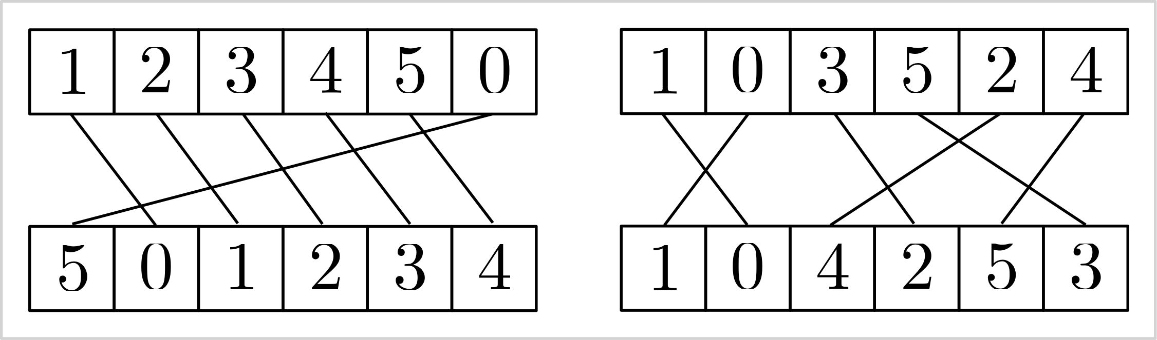 |
| :--------------------------------------------------------------------------------------------------: |
| Visualizing the stable matching induced by the `add_inverse` constraint. |
> [!WARNING]
>
> I generally advise against using the `add_element` and `add_inverse`
> constraints. While CP-SAT may have effective propagation techniques for them,
> these constraints can appear unnatural and complex. It's often more
> straightforward to model stable matching with binary variables $x_{ij}$,
> indicating whether $v_i$ is matched with $w_j$, and employing an
> `add_exactly_one` constraint for each vertex to ensure unique matches. If your
> model needs to capture specific attributes or costs associated with
> connections, binary variables are necessary. Relying solely on indices would
> require additional logic for accurate representation. Additionally, use
> non-binary variables only if the numerical value inherently carries semantic
> meaning that cannot simply be re-indexed.
## Advanced Modeling
After having seen the basic elements of CP-SAT, this chapter will introduce you
to the more complex constraints. These constraints are already focused on
specific problems, such as routing or scheduling, but very generic and powerful
within their domain. However, they also need more explanation on the correct
usage.
- [Tour Constraints](#04-modelling-circuit): `add_circuit`,
`add_multiple_circuit`, `add_reservoir_constraint_with_active`
- [Intervals](#04-modelling-intervals): `new_interval_var`,
`new_interval_var_series`, `new_fixed_size_interval_var`,
`new_optional_interval_var`, `new_optional_interval_var_series`,
`new_optional_fixed_size_interval_var`,
`new_optional_fixed_size_interval_var_series`,
`add_no_overlap`,`add_no_overlap_2d`, `add_cumulative`
- [Automaton Constraints](#04-modelling-automaton): `add_automaton`
- [Reservoir Constraints](#04-modelling-reservoir): `add_reservoir_constraint`,
- [Piecewise Linear Constraints](#04-modelling-pwl): Not officially part of
CP-SAT, but we provide some free copy&pasted code to do it.
### Circuit/Tour-Constraints
Routes and tours are essential in addressing optimization challenges across
various fields, far beyond traditional routing issues. For example, in DNA
sequencing, optimizing the sequence in which DNA fragments are assembled is
crucial, while in scientific research, methodically ordering the reconfiguration
of experiments can greatly reduce operational costs and downtime. The
`add_circuit` and `add_multiple_circuit` constraints in CP-SAT allow you to
easily model various scenarios. These constraints extend beyond the classical
[Traveling Salesman Problem (TSP)](https://en.wikipedia.org/wiki/Travelling_salesman_problem),
allowing for solutions where not every node needs to be visited and
accommodating scenarios that require multiple disjoint sub-tours. This
adaptability makes them invaluable for a broad spectrum of practical problems
where the sequence and arrangement of operations critically impact efficiency
and outcomes.
| 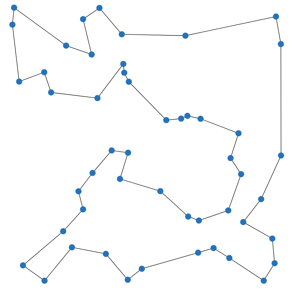 |
| :-------------------------------------------------------------------------------------------------------------------------------------------------: |
| The Traveling Salesman Problem (TSP) asks for the shortest possible route that visits every vertex exactly once and returns to the starting vertex. |
The Traveling Salesman Problem is one of the most famous and well-studied
combinatorial optimization problems. It is a classic example of a problem that
is easy to understand, common in practice, but hard to solve. It also has a
special place in the history of optimization, as many techniques that are now
used generally were first developed for the TSP. If you have not done so yet, I
recommend watching
[this talk by Bill Cook](https://www.youtube.com/watch?v=5VjphFYQKj8), or even
reading the book
[In Pursuit of the Traveling Salesman](https://press.princeton.edu/books/paperback/9780691163529/in-pursuit-of-the-traveling-salesman).
> [!TIP]
>
> If your problem is specifically the Traveling Salesperson Problem (TSP), you
> might find the
> [Concorde solver](https://www.math.uwaterloo.ca/tsp/concorde.html)
> particularly effective. For problems closely related to the TSP, a Mixed
> Integer Programming (MIP) solver may be more suitable, as many TSP variants
> yield strong linear programming relaxations that MIP solvers can efficiently
> exploit. Additionally, consider
> [OR-Tools Routing](https://developers.google.com/optimization/routing) if
> routing constitutes a significant aspect of your problem. However, for
> scenarios where variants of the TSP are merely a component of a larger
> problem, utilizing CP-SAT with the `add_circuit` or `add_multiple_circuit`
> constraints can be very beneficial.
| 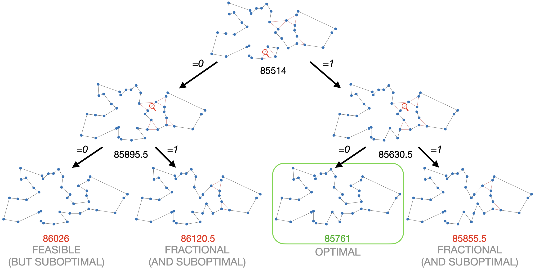 |
| :-------------------------------------------------------------------------------------------------------------------------------------------------------------------------------------------------------------------------------------------------------------------------------------------------------------------------------------------------------------------------------------------------------------------------: |
| This example shows why Mixed Integer Programming solvers are so good in solving the TSP. The linear relaxation (at the top) is already very close to the optimal solution. By branching, i.e., trying 0 and 1, on just two fractional variables, we not only find the optimal solution but can also prove optimality. The example was generated with the [DIY TSP Solver](https://www.math.uwaterloo.ca/tsp/D3/bootQ.html). |
#### `add_circuit`
The `add_circuit` constraint is utilized to solve circuit problems within
directed graphs, even allowing loops. It operates by taking a list of triples
`(u,v,var)`, where `u` and `v` denote the source and target vertices,
respectively, and `var` is a Boolean variable that indicates if an edge is
included in the solution. The constraint ensures that the edges marked as `True`
form a single circuit visiting each vertex exactly once, aside from vertices
with a loop set as `True`. Vertex indices should start at 0 and must not be
skipped to avoid isolation and infeasibility in the circuit.
Here is an example using the CP-SAT solver to address a directed Traveling
Salesperson Problem (TSP):
```python
from ortools.sat.python import cp_model
# Directed graph with weighted edges
dgraph = {(0, 1): 13, (1, 0): 17, ...(2, 3): 27}
# Initialize CP-SAT model
model = cp_model.CpModel()
# Boolean variables for each edge
edge_vars = {(u, v): model.new_bool_var(f"e_{u}_{v}") for (u, v) in dgraph.keys()}
# Circuit constraint for a single tour
model.add_circuit([(u, v, var) for (u, v), var in edge_vars.items()])
# Objective function to minimize total cost
model.minimize(sum(dgraph[(u, v)] * x for (u, v), x in edge_vars.items()))
# Solve model
solver = cp_model.CpSolver()
status = solver.solve(model)
if status in (cp_model.OPTIMAL, cp_model.FEASIBLE):
tour = [(u, v) for (u, v), x in edge_vars.items() if solver.value(x)]
print("Tour:", tour)
# Output: [(0, 1), (2, 0), (3, 2), (1, 3)], i.e., 0 -> 1 -> 3 -> 2 -> 0
```
This constraint can be adapted for paths by adding a virtual enforced edge that
closes the path into a circuit, such as `(3, 0, 1)` for a path from vertex 0 to
vertex 3.
#### Creative usage of `add_circuit`
The `add_circuit` constraint can be creatively adapted to solve various related
problems. While there are more efficient algorithms for solving the Shortest
Path Problem, let us demonstrate how to adapt the `add_circuit` constraint for
educational purposes.
```python
from ortools.sat.python import cp_model
# Define a weighted, directed graph with edge costs
dgraph = {(0, 1): 13, (1, 0): 17, ...(2, 3): 27}
source_vertex = 0
target_vertex = 3
# Add zero-cost loops for vertices not being the source or target
for v in [1, 2]:
dgraph[(v, v)] = 0
# Initialize CP-SAT model and variables
model = cp_model.CpModel()
edge_vars = {(u, v): model.new_bool_var(f"e_{u}_{v}") for (u, v) in dgraph}
# Define the circuit including a pseudo-edge from target to source
circuit = [(u, v, var) for (u, v), var in edge_vars.items()] + [
(target_vertex, source_vertex, 1)
]
model.add_circuit(circuit)
# Minimize total cost
model.minimize(sum(dgraph[(u, v)] * x for (u, v), x in edge_vars.items()))
# Solve and extract the path
solver = cp_model.CpSolver()
status = solver.solve(model)
if status in (cp_model.OPTIMAL, cp_model.FEASIBLE):
path = [(u, v) for (u, v), x in edge_vars.items() if solver.value(x) and u != v]
print("Path:", path)
# Output: [(0, 1), (1, 3)], i.e., 0 -> 1 -> 3
```
This approach showcases the flexibility of the `add_circuit` constraint for
various tour and path problems. Explore further examples:
- [Budget constrained tours](https://github.com/d-krupke/cpsat-primer/blob/main/examples/add_circuit_budget.py):
Optimize the largest possible tour within a specified budget.
- [Multiple tours](https://github.com/d-krupke/cpsat-primer/blob/main/examples/add_circuit_multi_tour.py):
Solve for $k$ minimal tours covering all vertices.
#### `add_multiple_circuit`
You can model multiple disjoint tours using several `add_circuit` constraints,
as demonstrated in
[this example](https://github.com/d-krupke/cpsat-primer/blob/main/examples/add_circuit_multi_tour.py).
If all tours share a common depot (vertex 0), the `add_multiple_circuit`
constraint is an alternative. However, this constraint does not allow you to
specify the number of tours, nor can it determine to which tour a particular
edge belongs. Therefore, the `add_circuit` constraint is often a superior
choice. Although the arguments for both constraints are identical, vertex 0
serves a unique role as the depot where all tours commence and conclude.
#### Performance of `add_circuit` for the TSP
The table below displays the performance of the CP-SAT solver on various
instances of the TSPLIB, using the `add_circuit` constraint, under a 90-second
time limit. The performance can be considered reasonable, but can be easily
beaten by a Mixed Integer Programming solver.
| Instance | # vertices | runtime | lower bound | objective | opt. gap |
| :------- | ---------: | ------: | ----------: | --------: | -------: |
| att48 | 48 | 0.47 | 33522 | 33522 | 0 |
| eil51 | 51 | 0.69 | 426 | 426 | 0 |
| st70 | 70 | 0.8 | 675 | 675 | 0 |
| eil76 | 76 | 2.49 | 538 | 538 | 0 |
| pr76 | 76 | 54.36 | 108159 | 108159 | 0 |
| kroD100 | 100 | 9.72 | 21294 | 21294 | 0 |
| kroC100 | 100 | 5.57 | 20749 | 20749 | 0 |
| kroB100 | 100 | 6.2 | 22141 | 22141 | 0 |
| kroE100 | 100 | 9.06 | 22049 | 22068 | 0 |
| kroA100 | 100 | 8.41 | 21282 | 21282 | 0 |
| eil101 | 101 | 2.24 | 629 | 629 | 0 |
| lin105 | 105 | 1.37 | 14379 | 14379 | 0 |
| pr107 | 107 | 1.2 | 44303 | 44303 | 0 |
| pr124 | 124 | 33.8 | 59009 | 59030 | 0 |
| pr136 | 136 | 35.98 | 96767 | 96861 | 0 |
| pr144 | 144 | 21.27 | 58534 | 58571 | 0 |
| kroB150 | 150 | 58.44 | 26130 | 26130 | 0 |
| kroA150 | 150 | 90.94 | 26498 | 26977 | 2% |
| pr152 | 152 | 15.28 | 73682 | 73682 | 0 |
| kroA200 | 200 | 90.99 | 29209 | 29459 | 1% |
| kroB200 | 200 | 31.69 | 29437 | 29437 | 0 |
| pr226 | 226 | 74.61 | 80369 | 80369 | 0 |
| gil262 | 262 | 91.58 | 2365 | 2416 | 2% |
| pr264 | 264 | 92.03 | 49121 | 49512 | 1% |
| pr299 | 299 | 92.18 | 47709 | 49217 | 3% |
| linhp318 | 318 | 92.45 | 41915 | 52032 | 19% |
| lin318 | 318 | 92.43 | 41915 | 52025 | 19% |
| pr439 | 439 | 94.22 | 105610 | 163452 | 35% |
There are two prominent formulations to model the Traveling Salesman Problem
(TSP) without an `add_circuit` constraint: the
[Dantzig-Fulkerson-Johnson (DFJ) formulation](https://en.wikipedia.org/wiki/Travelling_salesman_problem#Dantzig%E2%80%93Fulkerson%E2%80%93Johnson_formulation)
and the
[Miller-Tucker-Zemlin (MTZ) formulation](https://en.wikipedia.org/wiki/Travelling_salesman_problem#Miller%E2%80%93Tucker%E2%80%93Zemlin_formulation[21]).
The DFJ formulation is generally regarded as more efficient due to its stronger
linear relaxation. However, it requires lazy constraints, which are not
supported by the CP-SAT solver. When implemented without lazy constraints, the
performance of the DFJ formulation is comparable to that of the MTZ formulation
in CP-SAT. Nevertheless, both formulations perform significantly worse than the
`add_circuit` constraint. This indicates the superiority of using the
`add_circuit` constraint for handling tours and paths in such problems. Unlike
end users, the `add_circuit` constraint can utilize lazy constraints internally,
offering a substantial advantage in solving the TSP.
### Scheduling and Packing with Intervals
A special case of variables are the interval variables, that allow to model
intervals, i.e., a span of some length with a start and an end. There are fixed
length intervals, flexible length intervals, and optional intervals to model
various use cases. These intervals become interesting in combination with the
no-overlap constraints for 1D and 2D. We can use this for geometric packing
problems, scheduling problems, and many other problems, where we have to prevent
overlaps between intervals. These variables are special because they are
actually not a variable, but a container that bounds separately defined start,
length, and end variables.
There are four types of interval variables: `new_interval_var`,
`new_fixed_size_interval_var`, `new_optional_interval_var`, and
`new_optional_fixed_size_interval_var`. The `new_optional_interval_var` is the
most expressive but also the most expensive, while `new_fixed_size_interval_var`
is the least expressive and the easiest to optimize. All four types take a
`start=` variable. Intervals with `fixed_size` in their name require a constant
`size=` argument defining the interval length. Otherwise, the `size=` argument
can be a variable in combination with an `end=` variable, which complicates the
solution. Intervals with `optional` in their name include an `is_present=`
argument, a boolean indicating if the interval is present. The no-overlap
constraints, discussed later, apply only to intervals that are present, allowing
for modeling problems with multiple resources or optional tasks. Instead of a
pure integer variable, all arguments also accept an affine expression, e.g.,
`start=5*start_var+3`.
```python
model = cp_model.CpModel()
start_var = model.new_int_var(0, 100, "start")
length_var = model.new_int_var(10, 20, "length")
end_var = model.new_int_var(0, 100, "end")
is_present_var = model.new_bool_var("is_present")
# creating an interval whose length can be influenced by a variable (more expensive)
flexible_interval = model.new_interval_var(
start=start_var, size=length_var, end=end_var, name="flexible_interval"
)
# creating an interval of fixed length
fixed_interval = model.new_fixed_size_interval_var(
start=start_var,
size=10, # needs to be a constant
name="fixed_interval",
)
# creating an interval that can be present or not and whose length can be influenced by a variable (most expensive)
optional_interval = model.new_optional_interval_var(
start=start_var,
size=length_var,
end=end_var,
is_present=is_present_var,
name="optional_interval",
)
# creating an interval that can be present or not
optional_fixed_interval = model.new_optional_fixed_size_interval_var(
start=start_var,
size=10, # needs to be a constant
is_present=is_present_var,
name="optional_fixed_interval",
)
```
These interval variables are not useful on their own, as we could have easily
achieved the same with a simple linear constraint. However, CP-SAT provides
special constraints for these interval variables, that would actually be much
harder to model by hand and are also much more efficient.
CP-SAT offers the following three constraints for intervals:
`add_no_overlap`,`add_no_overlap_2d`, `add_cumulative`. `add_no_overlap` is used
to prevent overlaps between intervals on a single dimension, e.g., time.
`add_no_overlap_2d` is used to prevent overlaps between intervals on two
dimensions, e.g., for packing rectangles. `add_cumulative` is used to model a
resource constraint, where the sum of the demands of the overlapping intervals
must not exceed the capacity of the resource.
The `add_no_overlap` constraints takes a list of (optional) interval variables
and ensures that no two present intervals overlap.
```python
model.add_no_overlap(
interval_vars=[
flexible_interval,
fixed_interval,
optional_interval,
optional_fixed_interval,
# ...
]
)
```
The `add_no_overlap_2d` constraints takes two lists of (optional) interval and
ensures that for every `i` and `j` either `x_intervals[i]` and `x_intervals[j]`
or `y_intervals[i]` and `y_intervals[j]` do not overlap. Thus, both lists must
have the same length as `x_intervals[i]` and `y_intervals[i]` are considered
belonging together. If either `x_intervals[i]` or `y_intervals[i]` are optional,
the whole object is optional.
```python
model.add_no_overlap_2d(
x_intervals=[
flexible_interval,
fixed_interval,
optional_interval,
optional_fixed_interval,
# ...
],
y_intervals=[
flexible_interval,
fixed_interval,
optional_interval,
optional_fixed_interval,
# ...
],
)
```
The `add_cumulative` constraint is used to model a resource constraint, where
the sum of the demands of the overlapping intervals must not exceed the capacity
of the resource. An example could be scheduling the usage of certain energy
intensive machines, where the sum of the energy demands must not exceed the
capacity of the power grid. It takes a list of intervals, a list of demands, and
a capacity variable. The list of demands must have the same length as the list
of intervals, as the demands of the intervals are matched by index. As capacity
and demands can be variables (or affine expressions), quite complex resource
constraints can be modeled.
```python
demand_vars = [model.new_int_var(1, 10, f"demand_{i}") for i in range(4)]
capacity_var = model.new_int_var(1, 100, "capacity")
model.add_cumulative(
intervals=[
flexible_interval,
fixed_interval,
optional_interval,
optional_fixed_interval,
],
demands=demand_vars,
capacity=capacity_var,
)
```
> [!WARNING]
>
> Do not directly jump to intervals when you have a scheduling problem.
> Intervals are great if you actually have a somewhat continuous time or space
> that you need to schedule. If you have a more discrete problem, such as a
> scheduling problem with a fixed number of slots, you can often model this
> problem much more efficiently using simple Boolean variables and constraints.
> Especially if you can use domain knowledge to find clusters of meetings that
> cannot overlap, this can be much more efficient. If the scheduling is
> dominated by the transitions, your scheduling problem may actually be a
> routing problems, for which the `add_circuit` constraint is more suitable.
Let us examine a few examples of how to use these constraints effectively.
#### Scheduling for a Conference Room with Intervals
Assume we have a conference room and need to schedule several meetings. Each
meeting has a fixed length and a range of possible start times. The time slots
are in 5-minute intervals starting at 8:00 AM and ending at 6:00 PM. Thus, there
are $10 \times 12 = 120$ time slots, and we can use a simple integer variable to
model the start time. With fixed meeting lengths, we can use the
`new_fixed_size_interval_var` to model the intervals. The `add_no_overlap`
constraint ensures no two meetings overlap, and domains for the start time can
model the range of possible start times.
To handle input data, let us define a `namedtuple` to store the meeting and two
functions to convert between time and index.
```python
# Convert time to index and back
def t_to_idx(hour, minute):
return (hour - 8) * 12 + minute // 5
def idx_to_t(time_idx):
hour = 8 + time_idx // 12
minute = (time_idx % 12) * 5
return f"{hour}:{minute:02d}"
# Define meeting information using namedtuples
MeetingInfo = namedtuple("MeetingInfo", ["start_times", "duration"])
```
Then let us create a few meetings we want to schedule.
```python
# Meeting definitions
meetings = {
"meeting_a": MeetingInfo(
start_times=[
[t_to_idx(8, 0), t_to_idx(12, 0)],
[t_to_idx(16, 0), t_to_idx(17, 0)],
],
duration=120 // 5, # 2 hours
),
"meeting_b": MeetingInfo(
start_times=[
[t_to_idx(10, 0), t_to_idx(12, 0)],
],
duration=30 // 5, # 30 minutes
),
"meeting_c": MeetingInfo(
start_times=[
[t_to_idx(16, 0), t_to_idx(17, 0)],
],
duration=15 // 5, # 15 minutes
),
"meeting_d": MeetingInfo(
start_times=[
[t_to_idx(8, 0), t_to_idx(10, 0)],
[t_to_idx(12, 0), t_to_idx(14, 0)],
],
duration=60 // 5, # 1 hour
),
}
```
Now we can create the CP-SAT model and add the intervals and constraints.
```python
# Create a new CP-SAT model
model = cp_model.CpModel()
# Create start time variables for each meeting
start_time_vars = {
meeting_name: model.new_int_var_from_domain(
cp_model.Domain.from_intervals(meeting_info.start_times),
f"start_{meeting_name}",
)
for meeting_name, meeting_info in meetings.items()
}
# Create interval variables for each meeting
interval_vars = {
meeting_name: model.new_fixed_size_interval_var(
start=start_time_vars[meeting_name],
size=meeting_info.duration,
name=f"interval_{meeting_name}",
)
for meeting_name, meeting_info in meetings.items()
}
# Ensure that now two meetings overlap
model.add_no_overlap(list(interval_vars.values()))
```
And finally, we can solve the model and extract the solution.
```python
# Solve the model
solver = cp_model.CpSolver()
status = solver.solve(model)
# Extract and print the solution
scheduled_times = {}
if status in (cp_model.OPTIMAL, cp_model.FEASIBLE):
for meeting_name in meetings:
start_time = solver.value(start_time_vars[meeting_name])
scheduled_times[meeting_name] = start_time
print(f"{meeting_name} starts at {idx_to_t(start_time)}")
else:
print("No feasible solution found.")
```
Doing some quick magic with matplotlib, we can visualize the schedule.
| 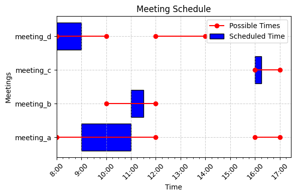 |
| :-----------------------------------------------------------------------------------------------------------------------------------: |
| A possible non-overlapping schedule for the above example. The instance is quite simple, but you could try adding some more meetings. |
#### Scheduling for Multiple Resources with Optional Intervals
Now, imagine we have multiple resources, such as multiple conference rooms, and
we need to schedule the meetings such that no two meetings overlap in the same
room. This can be modeled with optional intervals, where the intervals exist
only if the meeting is scheduled in the room. The `add_no_overlap` constraint
ensures that no two meetings overlap in the same room.
Because we now have two rooms, we need to create a more challenging instance
first. Otherwise, the solver may not need to use both rooms. We do this by
simply adding more and longer meetings.
```python
# Meeting definitions
meetings = {
"meeting_a": MeetingInfo(
start_times=[
[t_to_idx(8, 0), t_to_idx(12, 0)],
[t_to_idx(16, 0), t_to_idx(16, 0)],
],
duration=120 // 5,
),
"meeting_b": MeetingInfo(
start_times=[[t_to_idx(10, 0), t_to_idx(12, 0)]], duration=240 // 5
),
"meeting_c": MeetingInfo(
start_times=[[t_to_idx(16, 0), t_to_idx(17, 0)]], duration=30 // 5
),
"meeting_d": MeetingInfo(
start_times=[
[t_to_idx(8, 0), t_to_idx(10, 0)],
[t_to_idx(12, 0), t_to_idx(14, 0)],
],
duration=60 // 5,
),
"meeting_e": MeetingInfo(
start_times=[[t_to_idx(10, 0), t_to_idx(12, 0)]], duration=120 // 5
),
"meeting_f": MeetingInfo(
start_times=[[t_to_idx(14, 0), t_to_idx(14, 0)]], duration=240 // 5
),
"meeting_g": MeetingInfo(
start_times=[[t_to_idx(14, 0), t_to_idx(16, 0)]], duration=120 // 5
),
}
```
This time, we need to create an interval variable for each room and meeting, as
well as a Boolean variable indicating if the meeting is scheduled in the room.
We cannot use the same interval variable for multiple rooms, as otherwise the
interval would be present in both rooms.
```python
# Create the model
model = cp_model.CpModel()
# Create start time and room variables
start_time_vars = {
name: model.new_int_var_from_domain(
cp_model.Domain.from_intervals(info.start_times), f"start_{name}"
)
for name, info in meetings.items()
}
rooms = ["room_a", "room_b"]
room_vars = {
name: {room: model.new_bool_var(f"{name}_in_{room}") for room in rooms}
for name in meetings
}
# Create interval variables and add no-overlap constraint
interval_vars = {
name: {
# We need a separate interval for each room
room: model.new_optional_fixed_size_interval_var(
start=start_time_vars[name],
size=info.duration,
is_present=room_vars[name][room],
name=f"interval_{name}_in_{room}",
)
for room in rooms
}
for name, info in meetings.items()
}
```
Now