https://github.com/dabrokarol/atmorad-py
A 3D Monte Carlo simulation for radiative transfer.
https://github.com/dabrokarol/atmorad-py
atmospheric-science monte-carlo netcdf-files numpy physics-simulation python radiative-transfer
Last synced: about 2 months ago
JSON representation
A 3D Monte Carlo simulation for radiative transfer.
- Host: GitHub
- URL: https://github.com/dabrokarol/atmorad-py
- Owner: dabrokarol
- License: mit
- Created: 2026-04-23T22:53:33.000Z (3 months ago)
- Default Branch: main
- Last Pushed: 2026-05-27T23:07:26.000Z (about 2 months ago)
- Last Synced: 2026-05-27T23:12:10.580Z (about 2 months ago)
- Topics: atmospheric-science, monte-carlo, netcdf-files, numpy, physics-simulation, python, radiative-transfer
- Language: Python
- Homepage:
- Size: 7.21 MB
- Stars: 0
- Watchers: 0
- Forks: 0
- Open Issues: 5
-
Metadata Files:
- Readme: README.md
- License: LICENSE
Awesome Lists containing this project
README
# AtmoRad
## A vectorized Monte Carlo simulation of atmospheric radiative transfer.
[](https://pypi.org/project/atmorad-py/)
[](https://www.python.org/downloads/)
[](https://opensource.org/licenses/MIT)
[](#)
[](https://numpy.org/)
[](https://xarray.dev/)
[](https://github.com/h5netcdf/h5netcdf)
[](https://docs.astral.sh/uv/)
[](https://docs.astral.sh/ruff/)
[](https://docs.pytest.org/)
[](https://github.com/dabrokarol/atmorad-py/actions)
| **2D Surface absorption map** | **Sample photon paths** |
| :--- | :--- |
| 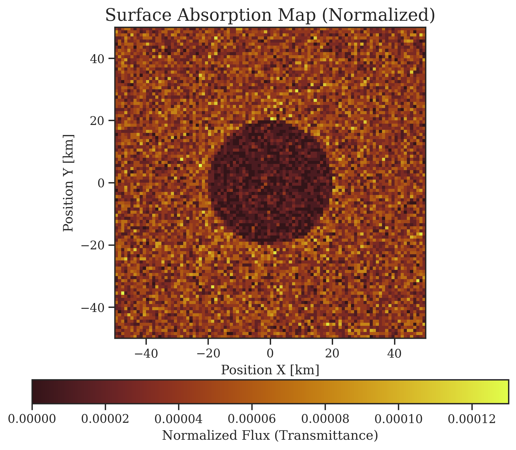 | 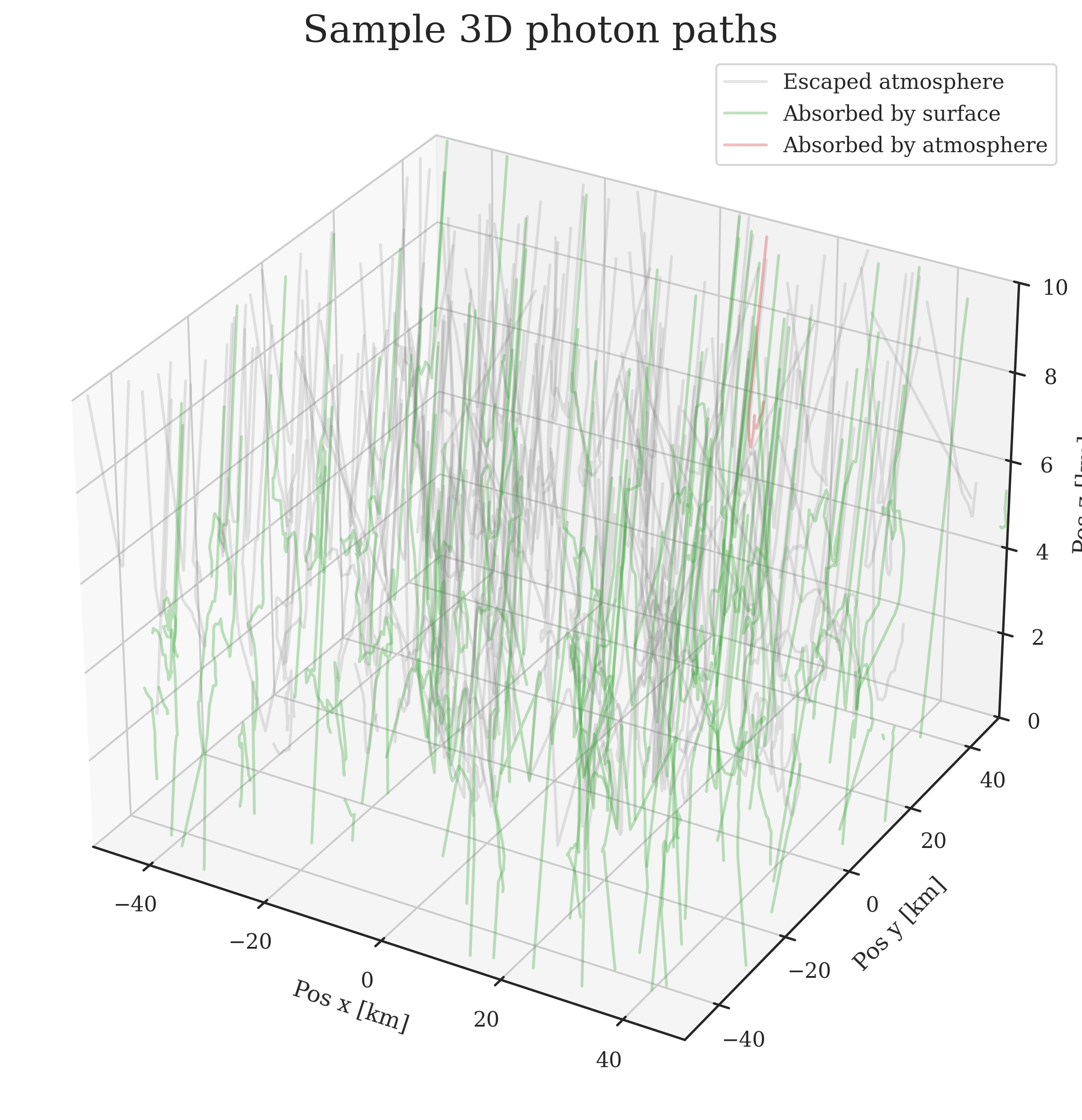 |
| **Vertical flux profile** | **Vertical absorption profile** |
| 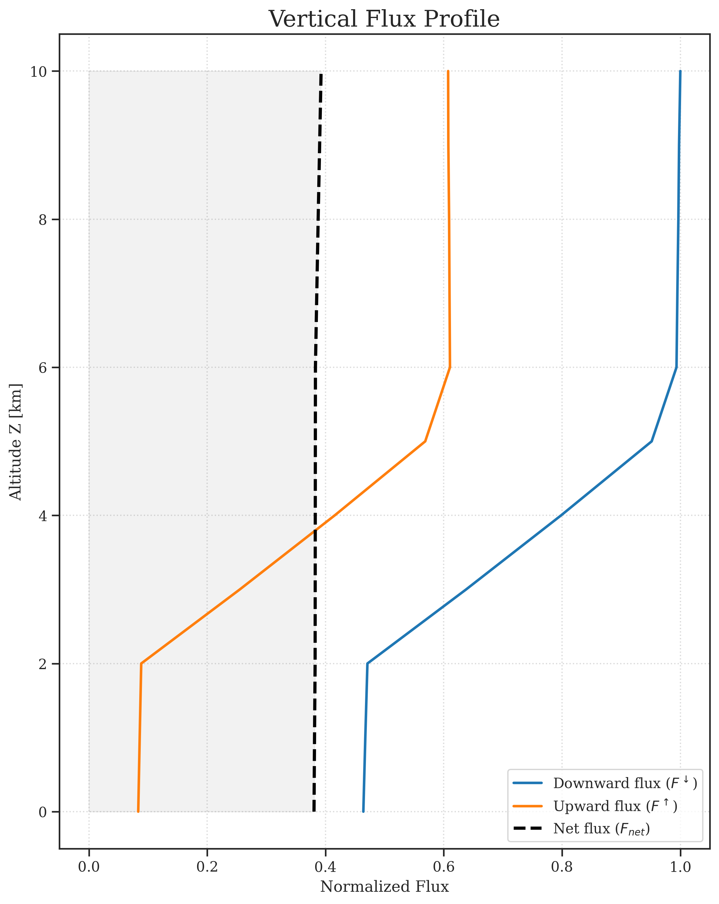| 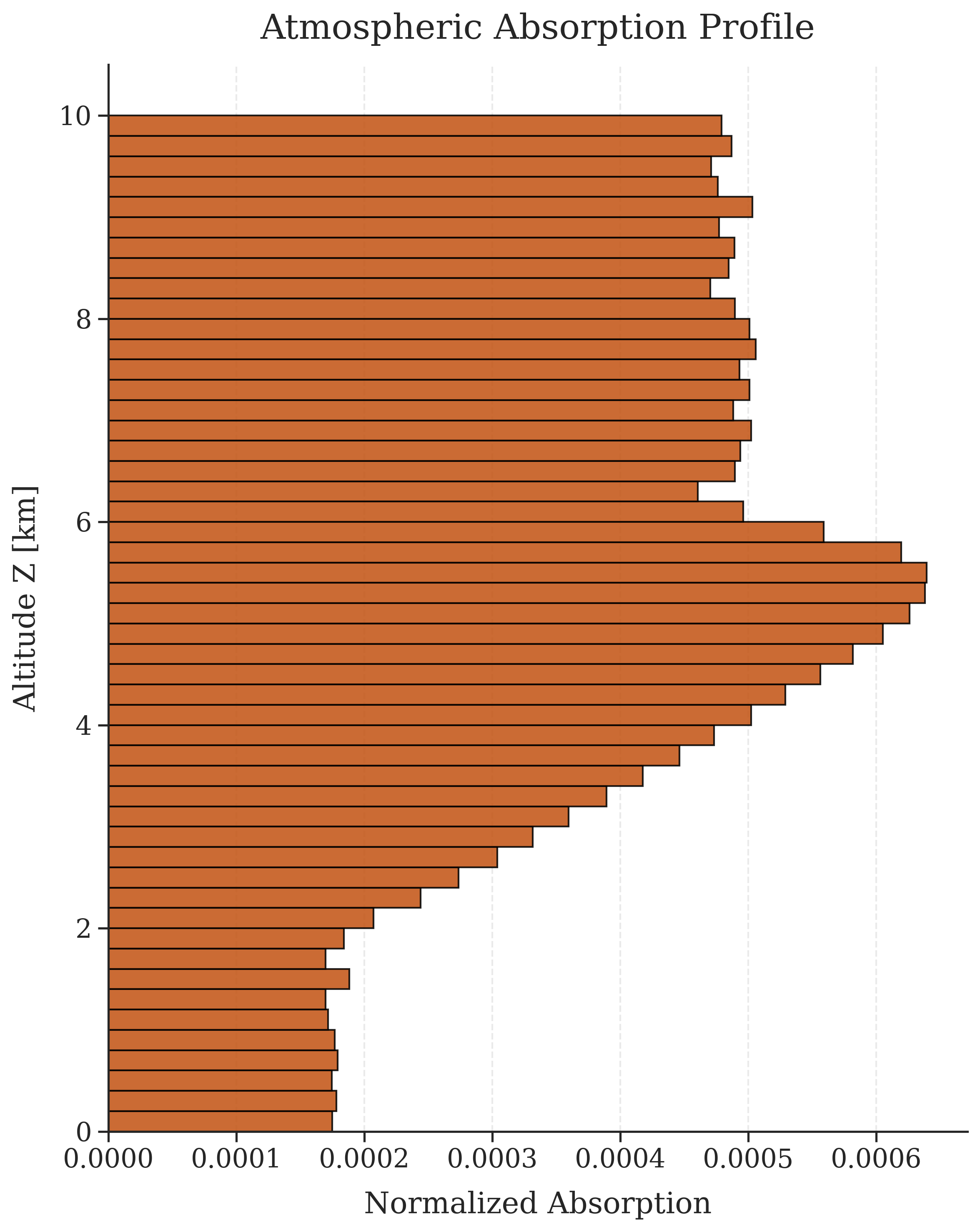 |
## Overview
AtmoRad is a Python tool for simulating the radiative transfer of monochromatic light over a mixed 2D surface and a plane-parallel atmosphere. I started it as a hobby project during lectures of Radiative Processes in the Atmosphere at the Faculty of Physics, University of Warsaw to learn computational physics and software development.
## Installation
Using [`uv`](https://docs.astral.sh/uv/getting-started/installation/) (Recommended for project isolation):
```bash
> uv tool install atmorad-py
```
Using `pip`:
```bash
> pip install atmorad-py
```
## Quickstart
Initialize a default configuration file in your current directory:
```bash
> atmorad --init
```
Run the simulation:
```bash
> atmorad simulation.toml
demo001/baseline: 100%|███████████████████████████████| 400000/400000 [00:10<00:00, 37632.74 photons/s]
---- Simulation Summary: demo001/baseline ----
Time: 10.63s (Total) | 35.49s (CPU)
Simulated Photons: 400_000
Energy Distribution:
Outgoing (TOA) : 64.35%
Surface Absorption : 33.57%
Atmospheric Absorption : 2.08%
------------------------------
Energy Conservation : 100.00%
Outputs saved to: results/demo001/
└─ atmorad_demo001_baseline.nc
```
*Check the `results/` directory for generated simulation artifacts and plots.*
## Features & Physical Model
- **Vectorized Monte Carlo Approach**: To fight Python's weak performance, uses **NumPy** and **multiprocessing** for fast and parallel processing of photons in large batches.
- **3D Radiative Transfer in Plane-Parallel Approximation**: The atmosphere consists of horizontally uniform layers, but photon paths are tracked in fully 3D space over a 2D surface.
- **Multi-Material Atmospheric Layers**: Layers can consist of multiple atmospheric materials simultaneously. Each material defines its own extinction coefficient, SSA, and phase function (built-in Rayleigh and Henyey-Greenstein, or custom).
- **Two Scattering Mechanisms**: Supports photon scattering using analytical inverse phase functions as well as numerical inverse CDFs for custom distributions.
- **Surface Reflections**: The surface consists of materials with specific albedos, predefined BRDF reflection models (`lambertian`, `specular`), and a `ProceduralMap` mapping material IDs to spatial coordinates.
- **Photon Properties**: Light is treated as monochromatic, non-polarized, weighted particles that can be scattered, reflected, and partially absorbed.
- **Checkpointing & Data Formats**: Supports resuming from checkpoints in case of interruption. Results are stored in the **NetCDF/HDF5** standard. Results are self-contained in a single `.nc` file.
## Roadmap
I'm planning to include more features in the future, such as:
- Delta tracking for arbitrary 3D cloud geometries.
- Wavelength-dependent optical properties of materials.
- Roughness parameter in specular reflection and other BRDF models.
- 3D surface topography.
- Spherical geometry for high zenith angles and whole-Earth simulations.
## Configuration
The simulation is controlled via a TOML configuration file (click to expand).
```toml
[metadata]
experiment_name = "demo001"
description = "A demo simulation of 3D radiative transfer over a heterogeneous surface."
[engine]
num_photons = 400_000
batch_size = 100_000 # photons will be processed in arrays of batch_size in parallel
random_seed = 42
cpu_cores = 4
resume_from_checkpoint = false
# Russian Roulette params
photon_weight_threshold = 1e-4
photon_survival_chance = 0.1 # 10% chance to survive with 10x multiplied weight
[source]
theta_sun_deg = 30 # solar zenith angle (0 = directly downwards)
phi_sun_deg = 0 # solar azimuth angle
wavelength_nm = 530 # only for reference, wavelength-dependent parameters are not implemented yet
[geometry]
domain_size_x_km = 100
domain_size_y_km = 100
boundary_condition = "periodic"
[detectors]
active = [ # list of supported detectors
"fate",
"path_tracking",
"vertical_flux",
"absorption_vertical",
"plane_flux",
"surface_absorption"
]
# spatial resolution for bins in detectors
vertical_profiles_resolution_km = 0.2
horizontal_maps_resolution_km = 1.0
num_full_paths = 200 # 200 photon paths will be saved to results
flux_maps_z_levels_km = [0.0, 4.0, 10.0] # planes at which vertical flux will be counted
[output]
save_plots = true
overwrite = true
path = 'results'
# --- material names and properties (can be added or changed) ---
[surface_materials.snow]
albedo = 0.85
reflection = {type = "lambertian"}
[surface_materials.ocean]
albedo = 0.01
reflection = {type = "specular", roughness = 0.0}
[atmosphere_materials.air]
extinction_coeff_per_km = 0.01 # optical density
ssa = 0.9
scattering = {type = "rayleigh"}
[atmosphere_materials.light_clouds]
extinction_coeff_per_km = 1
ssa = 0.999999 # almost no absorption, scattering
scattering = {type = "hg", g = 0.85} # g > 0 means forward scattering
[atmosphere_materials.dark_clouds]
extinction_coeff_per_km = 5
ssa = 0.999999
scattering = {type = "hg", g = 0.85}
# ___ atmospheric layers (bottom to top) ___
[[layer]] ## double square brackets are used for a list item
thickness_km = 2
components = [{material = "air", concentration = 1.0}]
[[layer]]
thickness_km = 4
components = [
{material = "air", concentration = 1.0},
{material = "dark_clouds", concentration = 0.9}
]
[[layer]]
thickness_km = 4
components = [{material = "air", concentration = 1.0}]
# [[layer]] ... more layers can be added
# ___ surface map configuration ___
# choose one surface map by commenting out the others
# [surface]
# name = "uniform"
# material = "snow"
[surface]
name = "circle"
radius_km = 20
material_in = "snow"
material_out = "ocean"
# [surface]
# name = "split_half_x"
# material_left = "snow"
# material_right = "ocean"
# [surface]
# name = "checkerboard"
# tile_size_km = 10
# material_a = "snow"
# material_b = "ocean"
# batch experiments
# append multiple [[scenario]] blocks (one per simulation) to run a series of experiments
# overrides the solar angle to 30 degrees
# [[scenario]]
# name = "sun_30"
# source.theta_sun_deg = 30
# overrides both the solar angle and the photon count
# [[scenario]]
# name = "sun_60"
# engine.num_photons = 500_000
# source.theta_sun_deg = 60
# overrides russian roulette treshold
# [[scenario]]
# name = "no_roulette"
# engine.photon_weight_threshold = 0.0
```
### Running Multiple Scenarios:
You can run multiple scenarios by appending [[scenario]] blocks to the end of your TOML file. You can override any base variable using dot-notation.
```toml
# Overrides the solar angle to 30 degrees
[[scenario]]
name = "sun_30"
source.theta_sun_deg = 30
# Overrides both the solar angle and the photon count
[[scenario]]
name = "sun_60"
engine.num_photons = 500_000
source.theta_sun_deg = 60
```
## Custom Physics & Geometries
AtmoRad allows you to easily inject custom surface maps, reflection models, scattering phase functions, and detectors using decorators (click to expand).
### Custom Materials and Geometries
```python
import numpy as np
import atmorad
from atmorad import (
Scattering,
register_reflection,
register_scattering,
register_surface_map,
)
from atmorad.constants import X
from atmorad.physics import orientation
# 1. Register a custom surface map
@register_surface_map("custom-stripe-y", ["material_name_a", "material_name_b"])
def stripe_y_map(pos: np.ndarray, stripe_width_km: float) -> np.ndarray:
"""Returns 0 for material A, 1 for material B."""
grid_x = np.mod(pos[X], stripe_width_km)
return np.where(grid_x < (stripe_width_km / 2.0), 0, 1)
# 2. Register a custom surface reflection
@register_reflection("custom-reflection")
def custom_reflection(
direction: np.ndarray, rand_1: np.ndarray, rand_2: np.ndarray, param_1: float, param_2: float
) -> np.ndarray:
"""
Cosine-weighted hemispherical sampling.
Note: param_1 and param_2 are injected directly from TOML.
"""
cos_theta = np.sqrt(rand_1)
sin_theta = np.sqrt(1.0 - rand_1)
phi = rand_2 * 2 * np.pi
return orientation(cos_theta, sin_theta, np.cos(phi), np.sin(phi))
# 3.a. Register a custom numerical scattering phase function
@register_scattering("custom-scattering")
class CustomScattering(Scattering):
def __init__(self, g: float):
cos_grid = np.linspace(-1, 1, 1000)
# Calculate the probability density function
pdf = (1 - g**2) / (2 * (1 + g**2 - 2 * g * cos_grid) ** 1.5)
# Calling base class automatically normalizes and builds the numerical inverse
super().__init__(pdf_array=pdf)
# 3.b. Register a custom analytical scattering phase function (usually better performance)
@register_scattering("custom-scattering-b")
def custom_scattering(rand_1, rand_2, g: float):
cos_theta = 2.0 * rand_1 - 1.0
sin_theta = np.sqrt(1.0 - cos_theta**2)
phi = 2.0 * np.pi * rand_2
return np.array((cos_theta, sin_theta, np.cos(phi), np.sin(phi)))
if __name__ == "__main__":
# 4. Run the experiment
results = atmorad.run("simulation.toml")
```
To use these in `simulation.toml`:
```toml
[atmosphere_materials.custom-atm-material]
ssa = 0.9
scattering = {type = "custom-scattering", g = 0.8}
[surface_materials.custom-surf-material-a]
albedo = 0.5
reflection = {type = "custom-reflection", param_1 = 2, param_2 = 1.3}
[surface]
name = "custom-stripe-y"
stripe_width_km = 5.0
material_name_a = "custom-surf-material-a"
material_name_b = "ocean"
```
### Custom Detectors
You can define custom detectors that record photon movement, interaction (scattering, reflection) and termination. It is also possible to create a class inheriting from 'BaseResult' which will allow for easy auto-saving to netcdf.
```python
from dataclasses import dataclass
import numpy as np
import atmorad
from atmorad import (
BaseDetector,
BaseResult,
Scene,
SimConfig,
nc_attr,
register_detector,
)
# 1. Define the result structure using AtmoRad's field wrappers
@dataclass(slots=True)
class FateResult(BaseResult):
energy_absorbed_surface: float = nc_attr(normalize=True)
energy_absorbed_atmosphere: float = nc_attr(normalize=True)
energy_outgoing_toa: float = nc_attr(normalize=True)
# 2. Implement the detector logic
@register_detector("fate", FateResult)
class FateDetector(BaseDetector):
def __init__(self, scene: Scene, config: SimConfig):
self.absorbed_surface = 0.0
self.absorbed_atmosphere = 0.0
self.escaped_toa = 0.0
self.scene = scene
def record_interaction(self, batch, scatter_mask, surface_mask):
# Calculate deposited energy by subtracting the photon's new weight from its old weight.
if np.any(scatter_mask):
deposited = batch.old_weight[scatter_mask] - batch.weight[scatter_mask]
self.absorbed_atmosphere += np.sum(deposited)
if np.any(surface_mask):
deposited = batch.old_weight[surface_mask] - batch.weight[surface_mask]
self.absorbed_surface += np.sum(deposited)
def record_termination(self, batch, terminated_mask):
if not np.any(terminated_mask):
return
term_pos = batch.pos[:, terminated_mask]
term_weight = batch.weight[terminated_mask]
escaped_toa_mask = self.scene.above_toa(term_pos)
if np.any(escaped_toa_mask):
self.escaped_toa += np.sum(term_weight[escaped_toa_mask])
def get_results(self) -> FateResult:
return FateResult(
energy_absorbed_surface=self.absorbed_surface,
energy_absorbed_atmosphere=self.absorbed_atmosphere,
energy_outgoing_toa=self.escaped_toa,
)
if __name__ == "__main__":
# 3. Run the simulation
results = atmorad.run("simulation.toml")
```
## Loading Results
Simulation results and configurations can be loaded in Python (e.g., Jupyter Notebook) for further analysis in two ways:
### 1. Using the built-in `atmorad.load()`
This method loads both the exact configuration used (a `SimConfig` instance) and results of the simulation (a `SimResults` instance).
```python
import matplotlib.pyplot as plt
import atmorad
# Load the completed simulation
results = atmorad.load("results/demo001/")
# Access physical data as NumPy arrays
map_2d = results.detector_results["surface_absorption"].surface_absorption_map_2d
# Analyze or plot
plt.imshow(map_2d)
plt.title(f"Flux Map for {results.config.metadata.experiment_name}")
plt.show()
```
### 2. Using standard NetCDF libraries
Because AtmoRad saves data in the standard NetCDF4/HDF5 format, you can read the `data.nc` file directly using libraries like `xarray` or `netCDF4`.
```python
import xarray as xr
# Open the NetCDF file directly
ds = xr.open_dataset("results/demo001/atmorad_demo001_baseline.nc", engine="h5netcdf")
# Access variables and attributes ({detector_name}_{attribute_name})
map_2d = ds["surface_absorption_surface_absorption_map_2d"].values
total_reflected_energy = ds.attrs["fate_energy_outgoing_toa"]
```
### 3. Extracting configuration file from results
Each data `.nc` file contains configuration data used to run the simulation. You can extract it by running:
```bash
atmorad --extract-config
```
This method created an __config.toml file in your working directory.
## Project Structure
- `engine/`: Handles photon batching and runs the main simulation loop.
- `physics/`: Contains rotation functions, scattering phase functions, and reflection models.
- `environment/`: Manages the environment (`Scene`, `Atmosphere`, `Surface`).
- `detectors/`: Implements photon tracking and result generation.
- `models/`: Defines base classes used throughout the program (and extensive 'results.py' for parsing netcdf).
- `output/`: Handles data IO and figure generation.
- `config/`: Parses `.toml` configuration files and constructs the simulation context.
- `cli.py`: Command-line interface entry point.
## References and Literature
- (in Polish) Script for Lecture about [Radiative Processes in the Atmosphere](https://www.igf.fuw.edu.pl/~kmark/stacja/wyklady/ProcesyRadiacyjne/2013/WykladRadiacjaKlimat.pdf), Prof. K. Markowicz, Faculty of Physics, University of Warsaw, 2013.
## Acknowledgments
- I created this project inspired by the lectures on *Radiative Processes in the Atmosphere* by Prof. K. Markowicz, Faculty of Physics, University of Warsaw.
- I used Large Language Models for code debugging (quite a lot) and architectural decisions (e.g., how to structure the repository, which packages to use, how to save and read data).
## Contributing
Feel free to open an [Issue](https://github.com/dabrokarol/atmorad-py/issues) or submit a Pull Request to report bugs, suggest new features and ask questions :))