https://github.com/davidbhr/arnold
Python package to analyze cell forces using 3D Traction Force Microscopy assuming simple geometries
https://github.com/davidbhr/arnold
Last synced: 3 months ago
JSON representation
Python package to analyze cell forces using 3D Traction Force Microscopy assuming simple geometries
- Host: GitHub
- URL: https://github.com/davidbhr/arnold
- Owner: davidbhr
- License: mit
- Created: 2019-06-25T10:49:51.000Z (almost 6 years ago)
- Default Branch: master
- Last Pushed: 2022-12-23T12:38:51.000Z (over 2 years ago)
- Last Synced: 2025-01-22T21:29:02.526Z (4 months ago)
- Language: Python
- Homepage:
- Size: 27 MB
- Stars: 2
- Watchers: 0
- Forks: 0
- Open Issues: 0
-
Metadata Files:
- Readme: README.md
- License: LICENSE
Awesome Lists containing this project
README
# arnold
Arnold is a python package to analyze cellular forces using 3D traction force microscopy. It provides interfaces to the open-source finite element mesh generator [`Gmsh`](http://gmsh.info/) and to the network optimizer [`SAENO`](https://github.com/Tschaul/SAENO). Image processing functions can be used to extract matrix deformations. These deformations and the respective material properties can be transferred to simulations based on simple geometries (cylinder, sphere, dipole).
By assuming a simple cylindircal geometry, traction forces can for example be computed for muscle fibers with different geometries, different contractile strains and different tissue environments (*linear* and *non-linear* materials).
A scaling law, derived from such simulation in linear materials, enables computing forces just by the cell geometry, the strain and the material stiffness without the need of further individual simulations.
More detailed information can be found in the article: **[Measurement of skeletal muscle fiber contractility with high-speed traction microscopy](https://www.biorxiv.org/content/10.1101/733451v1)** (doi: https://doi.org/10.1101/733451)
## Installation
The current version of *arnold* can be installed by cloning this repository or by downloading the zipped version [here](https://github.com/davidbhr/arnold/zipball/master). By running the following command within the unzipped folder, all other required packages are automatically downloaded and installed.
```
pip install -e .
```
Then the module can be simply imported to python as following
```python
import arnold as ar
```
We still need to set up the interfaces to the open-source finite element mesh generator [`Gmsh`](http://gmsh.info/) and to the network optimizer [`SAENO`](https://github.com/Tschaul/SAENO) .
GMSH offers a python interface within the `Gmsh SDK` , that can be downloaded [here](http://gmsh.info/#Download)
or by simply running the following command: `pip install --upgrade gmsh-sdk`.
To find the equilibrium configuration for the applied boundary problem *arnold* uses the network optimizer [`SAENO`](https://github.com/Tschaul/SAENO). A precompiled version of `SAENO` for 64bit Windows systems can be downloaded [here](https://github.com/davidbhr/arnold/tree/master/docs/SAENO). To build SAENO on other platforms the project can be found [here](https://github.com/Tschaul/SAENO).
Now we need to tell Arnold one-time where `Gmsh` and `SAENO` are stored. Therefore we simply use:
```python
import arnold as ar
ar.utils.set_gmsh_path(r'C:\..\gmsh-4.3.0-Windows64-sdk')
ar.utils.set_saeno_path(r'C:\..\SAENO.exe')
```
Note: If the `Gmsh SDK` has been installed via `pip` the path to `Gmsh` does not have to be set at all.
> **UPDATE: Alternativley, we can use the purely python based implementation [saenopy](https://github.com/rgerum/saenopy). Therefore saeno does not have to be installed and the functions from `force.py` and `simulation.py` that are described below can be replaced by the equivalent functions within `force_saenopy.py` and `simulaton_saenopy.py`, e.g. using `ar.simulation_saenopy.cylindric_contraction(..)` instead of `ar.simulation.cylindric_contraction(..)`**
## Introduction
A application of arnold can look like the following measurement: Muscle fibers are embedded into a certain matrix environment (e.g. matrigel). Then a contraction is induced via electical stimulation. The deformation can be imaged e.g. via confocal, fluorescence or brightfield microscopy. Beads are embedded into the surrounding matrix to validate that the fibers are attached to the matrix environment and to trace the matrix deformations.
*In the Gif below a single flexor digitorum longus fiber embedded in matrigel is shown in the relaxed state and during different electrical stimuli*
.gif)
To measure the exerted muscle forces, we need the following information about the respective contraction and model an analogous experiment using a cylindrical inclusion:
- The **fiber length** and **fiber diameter** in relaxed state (can easily be measured from the raw images).
- The **strain** during the contraction (derived as (Relaxed_Length- Contracted_Length)/Relaxed_Length)
- The **material properties** of the surrounding matrix (see below for further details)
>For further applications arnold offers different geometries such as spheres or dipoles. Image processing functions may be used to create maximum projections from 3D stacks and extract deformations by using particle image velocity (OpenPiv) or by manual clicking lengths. With these information, SAENO simulations with individual geometry can be started. In addition also a full 3D regularization of all deformations from two given input stacks (in relaxed and contracted state) can be started. In the following, the method is first described by using cylindrical geometry
## Individual Simulation
A simulation can be splitted into three parts:
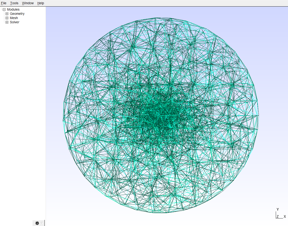
*__First__*, we need to build a mesh model of the geometry using GMSH. Here the fiber in the relaxed state is simulated as an inner cylindric inclusion with length *l_cyl* and diameter *d_cyl*, which is placed into a sphere with radius *r_outer* that simulates the matrix environment. Units are given in *µm* and the *length_factor* allows to tune the fineness of the mesh model (lower values correspond to a finer mesh. The element sizes are increased close to the cylindric inclusion by default)
```python
ar.mesh.cylindrical_inclusion(mesh_file=r'C/../Our_model.msh', d_cyl=30, l_cyl=300,
r_outer=2000, length_factor=0.2)
```
The resulting mesh can be displayed by using the following command:
```python
ar.mesh.show_mesh(r'C/../Our_model.msh')
```
*__Second__*, we apply corresponding boundary condition to our mesh and simulate the contraction of the cylinder using the network optimizer SAENO. We read in the *mesh_file* and apply a symetrical contraction with the given *strain* on the inner cylindrical inclusion with specific length *l_cyl* and diameter *d_cyl*. At the outer boundary of the bulk material we constrain the deformations to zero.
```python
ar.simulation.cylindric_contraction(simulation_folder=r'C/../Simulation', mesh_file=r'C/../Our_model.msh',
d_cyl=30, l_cyl=300, r_outer=2000, strain=0.1, ar.materials.matrigel_10mg_ml)
```
The material properties can be defined as following:
- To define a non-linear elastic material by it's linear stiffness (for instance 1000 Pa) use:
```python
ar.materials.linear_stiffness(1000)
```
- To define a specific Young's modulus (for instance 500 Pa) for a linear-elastic hydrogel (such as Matrigel) with a poission ratio of 0.25 (see [Steinwachs et al. (2016)](https://www.nature.com/articles/nmeth.3685)) use:
```python
ar.materials.youngs_modulus(500)
````
- To define non-linear materials use the `custom` material type:
```
ar.materials.custom(K_0, D_0, L_S, D_S)
```
Non-linear materials are characterized by four parameters:
- `K_0`: the linear stiffness (in Pa)
- `D_0`: the rate of stiffness variation during fiber buckling
- `L_S`: the onset strain for strain stiffening
- `D_S`: the rate of stiffness variation during strain stiffening
A full description of the non-linear material model and the parameters can be found in [Steinwachs et al. (2016)](https://www.nature.com/articles/nmeth.3685). Also "pre-configured" material types for Matrigel (10mg/ml) and collagen gels of three different concentrations (0.6, 1.2, and 2.4mg/ml) are available. Detailed protocols for reproducing these gels can be found in [Steinwachs et al. (2016)](https://www.nature.com/articles/nmeth.3685) and [Condor et al. (2017)](https://currentprotocols.onlinelibrary.wiley.com/doi/abs/10.1002/cpcb.24). Parameters for individual non-linear materials can be obtained by performing and fitting rheometer experiments with Saenopy as described [here](https://saenopy.readthedocs.io/en/latest/fit_material_parameters.html).
```python
ar.materials.collagen_06
ar.materials.collagen_12
ar.materials.collagen_24
ar.materials.matrigel_10mg_ml
```
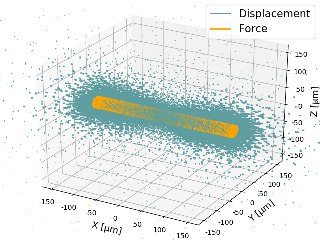
The results are stored in the set *simulation_folder*. For the nodes at the fiber surface we obtain the respective forces, which compensate for the fiber deformation, for the nodes in the bulk material we obtain the deformations, which are thereby generated in the surrounding matrix. More information about the output files of a simulation can be found in the [Wiki of the SAENO project](https://github.com/Tschaul/SAENO/wiki). The file `parameters.txt` contains all set parameters, that are used in the simulation.
*__Third__*, we compute the overall contractility from the resulting simulation by summing up the x-components of all forces on the cell surface from one end of the fiber to its center.
```python
ar.force.reconstruct_contractility(simulation_folder=r'C/../Simulation', d_cyl=30, l_cyl=300, r_outer=2000)
# or for a purely python-based implementation using saenopy
ar.force_saenopy.reconstruct_contractility(simulation_folder=r'C/../Simulation', d_cyl=30, l_cyl=300, r_outer=2000)
```
In an excel document the resulting contractility is saved under *'Contractility mean x-components'*. Further, the contractility is calculated considering the absolute forces instead of the x-components only and individually over the left half, the right half and total fiber volume. Additionally the residuum forces are calculated, which can be used to verify the simulation (forces at the outer boundary must compensate for the forces within the mesh moddel). For visualization and error detection an image of the deformtion- and force-field is stored.
*__All three abovementioned steps can be performed consecutively by using a single command. For an individual simulation you just need to execute the combined function:__*
```python
ar.experiment.cylindrical_inclusion_mesh_simulation_and_contractility(mesh_file=r'C/../Our_model.msh',
d_cyl=30,l_cyl=300, r_outer=2000, length_factor=0.2, simulation_folder=r'C/../Simulation',
strain=0.1, ar.materials.matrigel10)
```
Note: *mesh_file* and *simulation_folder* now only describe the desired directory and are created and used automatically. The arguments *iterations*, *step* and *conv_crit* allow to adjust the maximal number of iteration, the step width and the convergence criterium for the saeno simulation (see [Steinwachs et al. (2016)](https://www.nature.com/articles/nmeth.3685)).
Additionally *logfile=True* can be used to store the saeno system output in a text file.
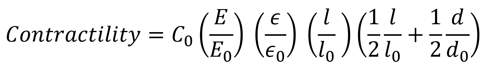
## Scaling law
For linear-elastic materials, the total contractility of muscle fibers scales linearly with matrix elasticity, linearly with fiber strain, quadratically with the fiber length and linearly with fiber diameter (see the article: **[Measurement of skeletal muscle fiber contractility with high-speed traction microscopy](https://www.biorxiv.org/content/10.1101/733451v1)** for more detailed information). Therefore we can estimate the contractility of a muscle fiber from the fiber diameter `d`, fiber length `l`, the fiber strain `s` during contraction (equals ε in the formula), and the Young’s modulus `E` of the surrounding Matrix by comparison with a reference simulation (denoted with zero subscripts) by uing the following simple scaling law (returns the contractility in µN):
```python
ar.force.scaling_law(d,l,s,E)
```
## Series
Additionally, Series of simulations can be performed for different diameters, lengths, strains and materials.
To start a series of simulation for a fixed fiber length, fixed strain and fixed stiffness for `n` fibers with diameters ranging from `d_cyl_min` to `d_cyl_max` in logarithmically spaced intervals, use:
```python
ar.experiment.simulation_series_diameter(d_cyl_min, d_cyl_max, l_cyl, n, r_outer,
length_factor, simulation_folder, strain, material, log_scaling=True, n_cores=None, dec=2):
```
Here *n_cores* defines the number of cores to run the simulations in paralell (for no entry the number of cores is detected by default) and `dec` defines the number of decimals for rounding. If `log_scaling` is `False`, linearly spaced intervals are used.
In a similar manner series for different lengths `ar.experiment.imulation_series_lengths(..)`, different strains `ar.experiment.imulation_series_strains(..)` and different stiffness `ar.experiment.imulation_series_stiffness(..)` can be used.
For all of these, an Excel sheet with evaluated contractility is created again in the simulation folder.
To compare several simulations in a more convenient way, the following function scans a given directiory (including all subdirectories) for simulations and creates an overview of the main values (cell geometry, strain, contractility, etc..). We just need to insert the path and may add an comment, which is used to name the resulting Excel-sheet. An example of the resulting overview can be seen below.
```python
ar.experiment.evaluate_series(path, comment='')
```

## Different geometries
A set of different mesh geometries and simulations (sphere, cylinder, dipole) are predefined in *mesh.py* and *simulation.py*
## Image
Different image analysis functions are included in *image.py*.
`ar.image.projections()`: Calculated Maximum/Mean/Median Intensity projections of image stacks
`ar.image.piv_analysis()`: Computes deformations between 2 images by crosscorrelation using openpiv
`ar.image.click_length()`: Computes the length of clicked line for given input image and scale
## 3D Regularization
Functions to start a SAENO 3D force regularization of a contracted and relaxed image stack are given within *regularization.py*.
## Dependencies
*arnold* is tested on Python 3.6. It depends on `numpy`, `pandas`, `matplotlib` ,`os`, `time`,`__future__` and `subprocess`. It is recommended to use the Anaconda distribution of Python. Windows users may also take advantage of pre-compiled binaries for all dependencies, which can be found at [Christoph Gohlke's page](http://www.lfd.uci.edu/~gohlke/pythonlibs/).
## License
The `arnold` package itself is licensed under the [MIT License](https://github.com/davidbhr/arnold/blob/master/LICENSE). Everything is provided "as is", without any warranty of any kind, express or implied, including but not limited to the warranties of merchantability, fitness for a particular purpose and noninfringement.