https://github.com/devinterview-io/feature-engineering-interview-questions
🟣 Feature Engineering interview questions and answers to help you prepare for your next machine learning and data science interview in 2024.
https://github.com/devinterview-io/feature-engineering-interview-questions
ai-interview-questions coding-interview-questions coding-interviews data-science data-science-interview data-science-interview-questions data-scientist-interview feature-engineering feature-engineering-interview-questions feature-engineering-questions feature-engineering-tech-interview interview-practice interview-preparation machine-learning machine-learning-and-data-science machine-learning-interview machine-learning-interview-questions software-engineer-interview technical-interview-questions
Last synced: 4 months ago
JSON representation
🟣 Feature Engineering interview questions and answers to help you prepare for your next machine learning and data science interview in 2024.
- Host: GitHub
- URL: https://github.com/devinterview-io/feature-engineering-interview-questions
- Owner: Devinterview-io
- Created: 2024-01-08T09:59:03.000Z (over 2 years ago)
- Default Branch: main
- Last Pushed: 2024-01-08T10:19:40.000Z (over 2 years ago)
- Last Synced: 2025-03-30T22:15:48.342Z (over 1 year ago)
- Topics: ai-interview-questions, coding-interview-questions, coding-interviews, data-science, data-science-interview, data-science-interview-questions, data-scientist-interview, feature-engineering, feature-engineering-interview-questions, feature-engineering-questions, feature-engineering-tech-interview, interview-practice, interview-preparation, machine-learning, machine-learning-and-data-science, machine-learning-interview, machine-learning-interview-questions, software-engineer-interview, technical-interview-questions
- Size: 16.6 KB
- Stars: 8
- Watchers: 1
- Forks: 1
- Open Issues: 0
-
Metadata Files:
- Readme: README.md
Awesome Lists containing this project
README
# Top 50 Feature Engineering Interview Questions in 2026

#### You can also find all 50 answers here 👉 [Devinterview.io - Feature Engineering](https://devinterview.io/questions/machine-learning-and-data-science/feature-engineering-interview-questions)
## 1. What is _feature engineering_ and how does it impact the performance of _machine learning models_?
**Feature engineering** is an essential part of building robust machine learning models. It involves selecting and transforming **input variables** (features) to maximize a model's predictive power.
### Feature Engineering: The Power Lever for Models
1. **Dimensionality Reduction**: High-performing models often work better with fewer, more impactful features. Techniques like **PCA** (Principal Component Analysis) and **t-SNE** (t-distributed Stochastic Neighbor Embedding) help visualize and choose top features.
2. **Feature Standardization and Scaling**: Data imbalance, where some features may have much wider ranges than others, can cause models like k-NN to favor certain features. Techniques like **z-score** standardization or **min-max scaling** ensure equal feature representation.
3. **Feature Selection**: Some features might not contribute significantly to the model's predictive power. Tools like **correlation matrices**, **forward/backward selection**, or specialized algorithms like **LASSO** and **Elastic Net** can help choose the most affective ones.
4. **Polynomial Features**: Sometimes, the nature of a relationship between a feature and a target variable is not linear. Codifying this as powers of features (like $x^2$ or $x^3$ ), can make the model more flexible.
5. **Feature Crosses**: In some cases, the relationship between features and the target is more nuanced when certain feature combinations are considered. **Polynomial Features** creates such combinations, enhancing the model's performance.
6. **Feature Embeddings**: Raw data could have too many unique categories (like user or country names). **Feature embeddings** **condense** this data into vectors of lower dimensions. This simplifies categorical data representation.
7. **Missing Values Handling**: Many algorithms can't handle **missing values**. Techniques for imputing missing values such as using the mean, median, or most frequent value, or even predicting the missing values, are important for model integrity.
8. **Feature Normality**: Some algorithms, including linear and logistic regression, expect features to be normally distributed. **Data transformation techniques** like the Box-Cox and Yeo-Johnson transforms ensure this conformance.
9. **Temporal Features**: For datasets with time-dependent relationships, features like this season's sale figures can improve prediction.
10. **Text and Image Features**: Dealing with non-numeric data, such as natural language or images, often requires specialized pre-processing techniques before these features can be generically processed. Techniques like **word embeddings** or **TF-IDF** enable machine learning models to work with text data, while **convolutional neural networks (CNNs)** are used for image feature extraction.
11. **Categorical Feature Handling**: Features with non-numeric representations, such as "red", "green", and "blue" in items' colors, might need to be converted to a numeric format (often via "one-hot encoding") before input to a model.
### Code Example: Feature Engineering Steps
Here is the Python code:
```python
from sklearn import datasets
import pandas as pd
# Load the iris dataset
iris = datasets.load_iris()
iris_df = pd.DataFrame(iris.data, columns=iris.feature_names)
# Perform feature selection
from sklearn.feature_selection import SelectKBest
from sklearn.feature_selection import chi2
X_new = SelectKBest(chi2, k=2).fit_transform(iris_df, iris.target)
# Create interaction terms using PolynomialFeatures
from sklearn.preprocessing import PolynomialFeatures
interaction = PolynomialFeatures(degree=2, include_bias=False, interaction_only=True)
X_interact= interaction.fit_transform(iris_df)
# Normalization with MinMaxScaler
from sklearn.preprocessing import MinMaxScaler
scaler = MinMaxScaler()
X_normalized = scaler.fit_transform(iris_df)
# Categorical feature encoding using One-Hot Encoding
from sklearn.preprocessing import OneHotEncoder
ohe = OneHotEncoder(sparse=False)
iris_encoded = ohe.fit_transform(iris_df[['species']])
# Show results
print("Selected Features after Chi2: \n", X_new)
print("Interaction Features using PolynomialFeatures: \n", X_interact)
```
## 2. List different types of _features_ commonly used in _machine learning_.
**Feature selection** is one of the most crucial aspects of machine learning. The process helps you identify and utilize the most relevant features, thereby improving the model's accuracy while reducing computational requirements.
### Categories of Features
#### Basic Categories
1. **Homogeneous features**: This includes multiple instances of the same feature for different sub-populations. An example would be a dataset of restaurants with separate ratings for food, service, and ambiance.
2. **Heterogeneous features**: These encompass a mix of different feature types within a single dataset. A prime instance would be a dataset for healthcare with numerical data (age, blood pressure), categories (diabetes type), binary data (gender), textual data (notes from patient visits), and dates (admission and discharge dates).
#### Advanced Categories
1. **Aggregated and Composite Features**: These are features that are derived from existing features. For example, an aggregated feature could be the mean of a set of numerical values, whereas a composite feature might be a concatenation of two text fields.
2. **Transformed Features**: These are features that have been mathematically altered but originate from the raw data. Common transformations include taking the square root or the logarithm.
3. **Latent (Hidden) Features**: These aren't directly observed within the dataset but are inferred. For instance, in collaborative filtering for recommendation systems, the tastes and preferences of users or the attributes of items can be thought of as latent features.
4. **Embedded Features**: These describe the technique of using one dataset as a feature within another. This can be a foundational part of multi-view learning, where data is described from multiple perspectives. An example could be using user characteristics as a feature in a user-item recommendation system, alongside data that captures user-item interactions.
### Techniques of Feature Engineering
#### High-Cardinality Texts
- **Technique**: Convert the texts to word vectors using techniques like TF-IDF or word embeddings.
- **Use Case**: Natural language features such as product descriptions or user reviews.
#### Categorical Features
- **Technique**: One-hot encoding or techniques like target encoding and weight of evidence for binary classification.
- **Use Case**: Gender, education level, or any other feature with limited categories.
#### Temporal Features
- **Technique**: Extract relevant information like hour of day, day of week, or time since an event.
- **Use Case**: Predictions that require a temporal aspect, like predicting traffic or retail sales.
#### Image Features
- **Technique**: Apply techniques from image processing such as edge detection, color histograms, or feature extraction through convolutional neural networks (CNNs).
- **Use Case**: Visual data like in object detection or facial recognition.
#### Missing Data
- **Technique**: Impute missing values using methods like mean or median imputation, or create a binary indicator of missingness.
- **Use Case**: Datasets with partially missing data.
#### Numerical Features
- **Technique**: Binning, scaling to a certain range, or z-score transformation.
- **Use Case**: Features like age, income, or any numerical values.
## 3. Explain the differences between _feature selection_ and _feature extraction_.
**Feature selection** and **feature extraction** are crucial steps in **dimensionality reduction**. They pave the way for more accurate and efficient machine learning models by streamlining input feature sets.
### Feature Selection
In **feature selection**, you identify a subset of the most significant features from the original feature space. This can be done using a variety of methods such as:
- **Filter Methods**: Directly evaluate features based on statistical metrics.
- **Wrapper Methods**: Utilize specific models to pick the best subset of features.
- **Embedded Methods**: Select features as part of the model training process.
Once you have reduced the feature set, you can use selected features in modeling tasks.
### Feature Extraction
**Feature extraction** involves transforming the original feature space into a reduced-dimensional one, typically using linear techniques like **PCA** or **factor analysis**. It achieves this by creating a new set of features that are **linear combinations of the original features**.
### Pitfalls of Overfitting and Interpretability
Both **feature selection** and **feature extraction** have the potential to suffer from overfitting issues.
- **Feature Selection**: If all features in a dataset are noisy or do not have any relationship with the target variable, feature selection methods can still mistakenly select some of them. This can lead to overfitting.
- **Feature Extraction**: With **unsupervised techniques** like PCA, the resulting features might not be the most relevant for predicting the target variable. Furthermore, the interpretability of these features could be lost.
### Hybrid Approaches
In practice, a combination of **feature selection** and **feature extraction** might offer the best results. This hybrid approach typically starts with **feature extraction** to reduce dimensionality, followed by **feature selection** to choose the most relevant features in the reduced space.
For example, in the banking sector, Principal Component Analysis (PCA) might be utilized to group correlated financial variables, allowing for better-informed **feature selection** for lending risk assessment. In marketing, **Word2vec**, which captures word semantics through the distribution of neighboring words, is often followed by **feature selection** to pinpoint the most influential keywords in social media sentiment analysis. In e-commerce, **Autoencoders** are fused with **feature selection** to streamline product image cataloging, optimizing customer recommendation processes.
This adaptive blend of strategies is known as "SEM" - Selection after Extraction or Feature Extraction followed by Feature Selection, designed to harness the advantages of both techniques and mitigate their limitations.
## 4. What are some common challenges you might face when _engineering features_?
**Feature engineering** is a critical component in the **machine learning pipeline**. While it holds great potential for refining models, it also presents several challenges.
### Challenges
#### Handling Missing Data
- Missing data can cause significant issues during model training. Deciding between deletion, mean or median imputation, or advanced techniques like multiple imputation is often tricky.
- For categorical variables, defining a separate category for missing values might introduce bias.
#### Discrete vs. Continuous Data
- Converting continuous variables to discrete during binning can lead to loss of statistical information.
- The choice of binning technique, such as equal-width or equal-frequency, can affect model performance.
#### Overfitting and Underfitting
- Over-engineering features to the extent that they capture noise or irrelevant patterns can lead to overfitting.
- Insufficient feature engineering, especially in complex tasks, can result in underfit models.
#### Data Leakage
- It's necessary to ensure that feature transformations, such as scaling or standardization, occur on the training data alone, without any information from the test set. Failing to do so can introduce data leakage, leading to overestimated model performance.
#### High Cardinality Categorical Features
- Excessive unique values in categorical features can inflate the feature space, making learning difficult.
- Techniques such as one-hot encoding might not be practical.
#### Legacy Data and Data Drift
- Features derived from historical data can become outdated when data distributions or business processes change.
- Continually monitoring a model's performance concerning the latest data is essential to avoid degradation over time due to data drift.
#### Text Data Challenges
- Textual features require careful preprocessing, including tokenization, stemming, or lemmatization to extract meaningful information.
- Constructing and embedding a comprehensive vocabulary while managing noisy text elements or rare terms poses a challenge.
## 5. Describe the process of _feature normalization_ and _standardization_.
**Feature normalization** and **standardization** help make datasets more **compatible** with various machine learning algorithms and provide a range of benefits.
### Importance
- **Algorithm Sensitivity**: Many ML algorithms are sensitive to different magnitude ranges. Normalizing features can mitigate this sensitivity.
- **Convergence and Performance**: Gradient-based algorithms, like linear regression and neural networks, can benefit from feature normalization in terms of convergence speed and model performance.
### Methods: Normalization and Standardization
The choice between normalization and standardization primarily depends on the nature of the data and the requirements of the algorithm.
1. **Normalization (Min-Max Scaling)**: Squeezes or stretches data features into a specified range, usually `[0, 1]`.
$$
x' = \dfrac{x - \min(x)}{\max(x) - \min(x)}
$$
2. **Standardization (Z-Score Scaling)**: Centers data around the mean and scales it to have a standard deviation of 1.
$$
x' = \dfrac{x - \mu}{\sigma}
$$
### Code Example: Normalization and Standardization
Here is the Python code:
```python
import pandas as pd
from sklearn.preprocessing import MinMaxScaler, StandardScaler
from sklearn.model_selection import train_test_split
from sklearn.linear_model import LogisticRegression
from sklearn.metrics import accuracy_score
# Load data
data = pd.read_csv('data.csv')
X, y = data.drop('target', axis=1), data['target']
# Split data
X_train, X_test, y_train, y_test = train_test_split(X, y, test_size=0.2)
# Initialize scalers
min_max_scaler = MinMaxScaler()
standard_scaler = StandardScaler()
# Normalize and standardize training data
X_train_normalized = min_max_scaler.fit_transform(X_train)
X_train_standardized = standard_scaler.fit_transform(X_train)
# Use the same transformations on test data
X_test_normalized = min_max_scaler.transform(X_test)
X_test_standardized = standard_scaler.transform(X_test)
# Train and evaluate models
logreg_normalized = LogisticRegression().fit(X_train_normalized, y_train)
logreg_standardized = LogisticRegression().fit(X_train_standardized, y_train)
print(f'Accuracy of model with normalized data: {accuracy_score(y_test, logreg_normalized.predict(X_test_normalized))}')
print(f'Accuracy of model with standardized data: {accuracy_score(y_test, logreg_standardized.predict(X_test_standardized))}')
```
## 6. Why is it important to understand the _domain knowledge_ while performing _feature engineering_?
**Feature engineering** often involves **pertinent domain knowledge**, drawing from the specific field or subject matter. Conscientiously integrating this expertise can yield more robust and interpretable models.
### Importance of Domain Knowledge in Feature Engineering
1. **Identifying Relevant Features**: Understanding the domain empowers data scientists to determine which features are most likely to be influential in model predictions.
2. **Minimizing Irrational Choices**: Relying purely on algorithms to select features can lead to inaccurate or biased models. Domain understanding can help mitigate these risks.
3. **Mitigating Adverse Effects from Data Issues**: Subject-matter expertise allows for targeted handling of common data issues like missing values or outliers.
4. **Improving Feature Transformation**: When you understand the data source, you can perform appropriate transformations and scaling, ensuring the model effectively captures meaningful patterns.
5. **Enhancing Model Interpretability**: Among the modern AI methods, interpreting complex models is a considerable challenge. By engineering features reflective of the domain, models can be more interpretable.
6. **Leveraging Data Sourcing Strategies**: Knowing the domain aids in better strategies for collecting additional data or leveraging external sources.
7. **Understanding Complexity**: Different domains carry varying levels of intrinsic complexity. Some may necessitate more intricate feature transformations, while others might benefit from simpler ones.
8. **Ensuring Feature Relevance and Adoptability**: Undergoing feature selection and engineering in tune with domain logic ensures model utility and acceptance by domain specialists.
### Practical Emphasis on Domain-Knowledge Driven Feature Engineering
- **Healthcare**: Employing disease-specific indicators as features can bolster model precision, particularly in diagnostics.
- **Finance**: Incorporating economic events or indicators can enrich models predicting stock movements.
- **E-Commerce**: Utilizing consumer behavior data, such as browsing habits and purchase history, can refine product suggestion models.
### Code Example: Domain-Informed Feature Selection
Here is the Python code:
```python
# Importing library
import pandas as pd
# Creating sample dataframe
data = {
'patient_id': range(1, 6),
'temperature': [98.2, 98.7, 104.0, 101.8, 99.0],
'cough_status': ['none', 'productive', 'dry', 'None', 'productive']
}
df = pd.DataFrame(data)
# Function to categorize fever based on clinical norms
def categorize_fever(temp):
if temp < 100.4:
return 'No Fever'
elif 100.4 <= temp < 102.2:
return 'Low-Grade Fever'
elif 102.2 <= temp < 104.0:
return 'Moderate-Grade Fever'
else:
return 'High-Grade Fever'
# Apply the category definition to the 'temperature' feature
df['fever_status'] = df['temperature'].apply(categorize_fever)
# Display the modified dataframe
print(df)
```
## 7. How does _feature scaling_ affect the performance of _gradient descent_?
**Feature scaling** holds significant implications for the performance of **gradient descent**, ranging from convergence speed to the likelihood of reaching the global minimum.
### Role of Feature Scaling in Gradient Descent
- **Convergence Speed**: Scaled features help reach the minimum quicker.
- **Loss Function Shape Stability**: Scaling ensures a smooth, symmetric loss function.
- **Algorithm Direction**: Without scaling, the algorithm may oscillate, slowing down the process.
### Key Methods for Feature Scaling
- **Min-Max Normalization**: Scales data within a range using a feature's minimum and maximum values.
$$
x_{scaled} = \dfrac{x - \min(x)}{\max(x) - \min(x)}
$$
- **Standardization**: Scales data to have a mean of 0 and a standard deviation of 1.
$$
x_{scaled} = \dfrac{x - \mu}{\sigma}
$$
### Code Example: Feature Scaling
Here is the Python code:
```python
import numpy as np
# Input data
data = np.array([[1.1, 2.2, 3.3],
[4.4, 5.5, 6.6],
[7.7, 8.8, 9.9]])
# Min-Max Normalization
min_val = np.min(data, axis=0)
max_val = np.max(data, axis=0)
scaled_minmax = (data - min_val) / (max_val - min_val)
# Standardization
mean_val = np.mean(data, axis=0)
std_val = np.std(data, axis=0)
scaled_std = (data - mean_val) / std_val
# Visualize
print("Data:\n", data)
print("\nMin-Max Normalized:\n", scaled_minmax)
print("\nStandardized:\n", scaled_std)
```
## 8. Explain the concept of _one-hot encoding_ and when you might use it.
**One-Hot Encoding** is a technique used to represent categorical data as binary vectors. This approach is typically used when the data lacks ordinal relationship, meaning there is no inherent order or ranking among the categories.
### How It Works
Here are the steps involved in One-Hot Encoding:
1. **Identify Categories**: Determine the unique categories present in the dataset, resulting in $N$ categories.
2. **Create Binary Vectors**: Assign a binary vector to each category, where each position in the vector represents a category. Here, $N = 3$:
- **Category A**: [1, 0, 0]
- **Category B**: [0, 1, 0]
- **Category C**: [0, 0, 1]
3. **Represent Entries**: For each data instance, replace the categorical value with its corresponding binary vector.
### Use-Cases
1. **Text Data**: For tasks like natural language processing, where words need to be converted into numeric form for machine learning algorithms.
2. **Categorical Variables**: Used in predictive modeling, especially when categories have no inherent order.
3. **Tree-Based Models**: Such as decision trees, which perform well with one-hot encoded inputs.
4. **Neural Networks**: Certain use-cases and network architectures warrant one-hot encoding, such as when dealing with an output layer from a network trained in a multi-class classification role.
5. **Linear Models**: Useful when working with regression and classification models, especially when using regularization methods.
### Code Example: One-Hot Encoding with scikit-learn
Here is the Python code:
```python
from sklearn.preprocessing import OneHotEncoder
import pandas as pd
# Sample data
data = pd.DataFrame({'fruit': ['apple', 'banana', 'cherry']})
# Initialize OneHotEncoder
encoder = OneHotEncoder()
# Transform and showcase results
onehot_encoded = encoder.fit_transform(data[['fruit']]).toarray()
print(onehot_encoded)
```
## 9. What is _dimensionality reduction_ and how can it be beneficial in _machine learning_?
**Dimensionality Reduction** is a data preprocessing technique that offers several benefits in machine learning, such as improving computational efficiency, minimizing overfitting, and enhancing data visualization.
### Key Methods
#### Feature Selection
This method involves choosing a subset of the most relevant features while eliminating less important or redundant ones. Techniques in both statistical and machine learning domains can be used for feature selection, such as univariate feature selection, recursive feature elimination, and lasso.
#### Feature Extraction
Here, new features are created as combinations of original ones, a process often referred to as "projection." Linear methods like Principal Component Analysis (PCA) are a common choice, though nonlinear models like autoencoders and kernel PCA are also available.
### Algorithmic Benefits
1. **Faster Computations**: Reducing feature count results in less computational resources required.
2. **Improved Model Performance**: By focusing on more relevant features, models become more accurate.
3. **Enhanced Generalization**: Overfitting is curbed as irrelevant noise is eliminated.
4. **Simplified Interpretability**: Models are easier to understand with a smaller feature set.
### Visual Representation
#### Scatter Plots
Before applying dimensionality reduction, it's challenging to visualize a dataset with more than three features. After dimensionality reduction, observing patterns and structures becomes feasible.
#### Clustering
After reducing dimensions, discerning clusters can be simpler. This is especially evident in datasets with many features, where clusters might not be perceptible in their original high-dimensional space.
### Mathematical Foundation: PCA
Principal Component Analysis is a linear dimensionality reduction method. Given $m$ data points with $n$ features, it finds $k$ orthogonal vectors, or principal components (PCs), that best represent the data. These PCs are used to transform the original $n$-dimensional input into a new $k$-dimensional space.
The first PC is the unit vector in the direction of maximum variance. The second PC is similarly defined but is orthogonal to the first, and so on.
#### Objective Function
The objective in PCA is to project the data onto a lower-dimensional space while retaining the maximum possible variance. This objective translates into an optimization problem.
Let $\mathbf{x}$ represent the original data matrix, where each row corresponds to a data point and each column to a feature. The variance of the projected data can be expressed as
$$
\text{variance} = \frac{1}{m} \sum_{i=1}^{m} (\mathbf{u}^\mathrm{T} \mathbf{x}^{(i)})^2
$$
where $\mathbf{u}$ is the vector representing the first principal component and $\mathbf{u}^\mathrm{T} \mathbf{x}^{(i)}$ is the projected data point. Maximizing this expression with respect to $\mathbf{u}$ is equivalent to maximizing the total variance along the direction of $\mathbf{u}$.
Principal Component Analysis achieves this maximization by solving the Eigenvalue-Eigenvector problem for the covariance matrix of $\mathbf{x}$. The Eigenvectors corresponding to the $n$ largest Eigenvalues are the sought-after principal components.
### Practical Application with Code
Here is the Python code:
```python
import numpy as np
from sklearn.decomposition import PCA
import matplotlib.pyplot as plt
from sklearn.preprocessing import StandardScaler
# Generate data
np.random.seed(0)
n = 100
X = np.random.normal(size=2*n).reshape(n, 2)
X = np.dot(X, np.random.normal(size=(2, 2)))
# Standardize Data
scaler = StandardScaler()
X_std = scaler.fit_transform(X)
# Apply PCA
pca = PCA(n_components=2)
X_pca = pca.fit_transform(X_std)
# Visualize before and after PCA
fig, axes = plt.subplots(1, 2, figsize=(10, 6))
axes[0].scatter(X_std[:, 0], X_std[:, 1])
axes[0].set_title('Before PCA')
axes[1].scatter(X_pca[:, 0], X_pca[:, 1])
axes[1].set_title('After PCA')
plt.show()
```
## 10. How do you handle _categorical variables_ in a _dataset_?
**Categorical variables** are non-numeric data types which can assume a limited, and usually fixed, number of values within a certain range. They can pose a challenge for many algorithms that expect numerical input. Here's how to tackle them:
### Handling Categorical Variables
#### 1. Ordinal Encoding
- **Description**: Assigns an integer value to each category based on specified order or ranking.
- **Considerations**: Appropriate for ordinal categories where relative ranking matters (e.g., "low," "medium," "high").
- **Code**:
```python
from sklearn.preprocessing import OrdinalEncoder
categories = ['low', 'medium', 'high']
ordinal_encoder = OrdinalEncoder(categories=[categories])
housing_cat_encoded = ordinal_encoder.fit_transform(housing_cat)
```
#### 2. One-Hot Encoding
- **Description**: Assigns each category to a unique binary (0 or 1) column of a feature vector.
- **Considerations**: Best for nominal categories without any inherent ranking or relationship.
- **Code**:
```python
from sklearn.preprocessing import OneHotEncoder
cat_encoder = OneHotEncoder()
housing_cat_1hot = cat_encoder.fit_transform(housing_cat)
```
#### 3. Dummy Variables
- **Description**: Converts each category into a binary column, leaving one category out, which becomes the baseline.
- **Considerations**: Used to avoid multicollinearity in models where the presence of multiple category columns can predict the baseline one.
- **Code**:
```python
housing_with_dummies = pd.get_dummies(data=housing, columns=['ocean_proximity'], prefix='op', drop_first=True)
```
#### 4. Feature Hashing
- **Description**: Transforms categories into a hash value of a specified length, which can reduce the dimensionality of the feature space.
- **Considerations**: Useful when memory or dimensionality is a significant concern. However, it's a one-way transformation that can lead to collisions.
- **Code**:
```python
from sklearn.feature_extraction import FeatureHasher
hash_encoder = FeatureHasher(n_features=5, input_type='string')
housing_cat_1hot = hash_encoder.fit_transform(housing_cat)
```
#### 5. Binary Encoding
- **Description**: More efficient alternative to one-hot encoding, particularly useful for high-cardinality categorical features. For example, when a feature has many categories, each unique category requires a separate column in a one-hot encoded feature. However, binary encoding only requires log2(N) bits to represent a feature with N categories.
- **Considerations**: It uses fewer features but may not be as interpretable as one-hot encoding.
- **Code**:
```python
import category_encoders as ce
binary_encoder = ce.BinaryEncoder(cols=['ocean_proximity'])
housing_bin_encoded = binary_encoder.fit_transform(housing)
```
#### 6. Target Encoding
- **Description**: Averages the target variable for each category to encode the category with its mean target value. Useful for data with large numbers of categories.
- **Considerations**: Risk of data leakage, necessitating careful validation and handling of out-of-sample data, such as cross-validation or applying target encoding within each fold.
- **Code**:
```python
from category_encoders import TargetEncoder
target_encoder = TargetEncoder()
housing_lm = target_encoder.fit_transform(housing, housing['ocean_proximity'], housing['median_house_value'])
```
#### 7. Probability Ratio Encoding
- **Description**: Calculates the probability of the target for each category and then divides the probability of the target within the category by the probability of the target within the entire dataset.
- **Considerations**: Useful for imbalanced datasets; however, similar to target encoding, can result in potential data leakage and needs to be handled with caution.
- **Code**:
```python
encoder = ce.ProbabilityRatioEncoder()
housing_encoded = encoder.fit_transform(housing, housing['ocean_proximity'], housing['median_house_value'] > 50000)
```
## 11. What are _filter methods_ in _feature selection_ and when are they used?
**Filter methods** are a simple, computationally efficient way to select the most relevant features using statistical measures. They evaluate features independently and are best suited for datasets with a large number of potential features.
### Filter Methods in Action
1. **Statistical Significance**: Features are evaluated based on statistical metrics such as **t-tests** (for continuous features in a two-group comparison), **ANOVA** (for more than two groups), and $\chi^2$ tests (for categorical features).
2. **Correlation Analysis**: Assess the strength of the relationship between two quantitative variables. **Pearson's correlation coefficient** is a frequently used metric.
3. **Information Theory**: Leverages concepts from information theory such as entropy and mutual information. **Mutual Information** quantifies the reduction in uncertainty for one variable given knowledge of another.
4. **L1 Regularization (Lasso)**: Also known as 'Lasso regression', L1 regularization can be incorporated in filter methods to **penalize low-impact features**.
5. **Consistency Methods**: These methods remove features that do not add valuable information in a step-by-step manner, such as the **McMaster Criterion**.
## 12. Explain what _wrapper methods_ are in the context of _feature selection_.
**Wrapper methods** represent a more sophisticated approach to **feature selection** that utilizes predictive models to assess the quality of subsets of features.
### Key Concepts
- **Model-Bounded Evaluation**: Wrapper methods perform feature selection within the context of a specific predictive model.
- **Exhaustive Search**: These methods evaluate all possible feature combinations or use a heuristic to approximate the best subset.
- **Direct Interaction with Model**: They involve the actual predictive algorithm, often using metrics like accuracy or AUC to determine feature subset quality.
### Types of Wrapper Methods
1. **Forward Selection**
Begins with an empty feature set and iteratively adds the best feature based on model performance. The process stops when further additions don't improve the model significantly.
2. **Backward Elimination**
Starts with the entire feature set and successively removes the least important feature, again based on model performance.
3. **Recursive Feature Elimination (RFE)**
Begins with all features, trains the model, and selects the least important features for elimination. It continues this process iteratively until the desired number of features is achieved.
### Strengths and Weaknesses
- **Strengths**:
- Less sensitive to feature interdependence.
- Directly employs the predictive model, making it suitable for complex, non-linear relationships.
- Often yields the best model performance among the three selection methods.
- **Weaknesses**:
- Generally computationally expensive because they evaluate multiple combinations.
- Might overfit data, especially with small datasets.
## 13. Describe _embedded methods_ for _feature selection_ and their benefits.
**Embedded methods** integrate feature selection within the model training process.
They are known for being:
- **Efficient**: Deploying these methods eliminates the need for EDA.
- **Accurate in Model-Feature Interactions**: They consider where and how features are used in the model for a more nuanced selection.
- **Conducive to Large Datasets**: These methods handle extensive data more capably than other feature selection techniques.
- **Automated**: They are integrated into the model, which enhances reproducibility.
### Techniques and Example Models
#### L1 Regularization (Lasso)
L1 regularization adds a penalty that encourages sparsity in the model's coefficients. This forces less informative or redundant features to have a coefficient of zero, effectively removing them from the model.
- **Example Model**: SGDClassifier from Scikit-Learn with `penalty='l1'`
- **Code**:
```python
from sklearn.linear_model import SGDClassifier
clf = SGDClassifier(loss='log', penalty='l1')
```
#### Decision Trees
Tree-based algorithms like Random Forest and Gradient Boosting Machines often leverage impurity-based feature importances derived from decision trees. These importances can be used to rank features based on their contribution to reducing impurity.
- **Example Model**: RandomForestClassifier from Scikit-Learn
- **Code**:
```python
from sklearn.ensemble import RandomForestClassifier
clf = RandomForestClassifier()
```
#### XGBoost and LightGBM Feature Selectors
XGBoost and LightGBM offer tools for **in-built feature selection**, especially during training, to improve model efficiency and generalization.
- **Example Model**: XGBoostClassifier from XGBoost
- **Code**:
```python
import xgboost as xgb
clf = xgb.XGBClassifier()
```
#### Permutation Importance
While not strictly embedded, permutation importance is a feature scoring technique often used with trees and ensembles.
Here's How It Works:
1. Train the model and record its performance on a validation set (**baseline performance**).
2. Shuffle one feature while keeping all others intact and evaluate the model's performance on the validation set.
3. The drop in the performance from the baseline represents the feature's importance: the larger the drop, the more important the feature.
It's especially useful for models that don't have built-in ways to assess feature importance, and it provides a straightforward understanding of a feature's usefulness.
- **Example Model**: Any tree-based model with scikit-learn, using the `permutation_importance` module.
- **Code**:
```python
from sklearn.inspection import permutation_importance
clf = RandomForestClassifier()
clf.fit(X_train, y_train)
result = permutation_importance(clf, X_val, y_val, n_repeats=10, random_state=42)
```
### Limitations and Best Practices
- **Model Dependence**: These techniques are closely tied to the abilities of specific models, meaning not all models can leverage them.
- **Initial Overhead**: The feature selection process may slow down initial model training.
- **Skills and Expertise Required**: Although these methods are relatively robust, some understanding of both the model and dataset are necessary to avoid unreliable outcomes.
For large datasets or when using algorithms that naturally employ these methods of feature selection, it might be preferable to let the model determine feature importance, as this can help save time and automate the process.
## 14. How does a feature's _correlation_ with the _target variable_ influence _feature selection_?
**Correlation with the Target Variable** is a crucial factor in determining the importance of features and subsequently in **feature selection**.
### Feature Importance
Utilizing correlation for feature importance has distinct advantages, especially when dealing with **supervised learning** tasks.
#### Key Metrics
1. **Pearson Correlation Coefficient ($r$)**: Measures the linear relationship between numerical variables.
2. **Point-Biserial Correlation**: Specialized for assessing relationships between a binary and a continuous variable.
3. **$R^2$ for Continous Response Variables**: Describes the proportion of variance explained by the model.
### Common Pitfalls with Correlation-Based Selection
- **Overlooking Nonlinear Relationships**: Correlation metrics, especially $r$, don't capture nonlinear associations effectively.
- **Ignoring Redundancy**: Even if two features have moderate correlations with the target variable, one might be redundant if they're highly correlated with each other.
- **Relevance in Ensemble Models**: While individual tree-based models may not require strongly correlated features, ensemble methods like **Random Forest** might still leverage the predictive power of these features.
### Code Example: Feature Importance with Correlation
Here is the Python code:
```python
import pandas as pd
from sklearn.datasets import load_boston
boston = load_boston()
data = pd.DataFrame(boston.data, columns=boston.feature_names)
data['PRICE'] = boston.target
correlated_features = abs(data.corr()['PRICE']).sort_values(ascending=False).index[1:]
correlated_features
```
## 15. What is the purpose of using _Recursive Feature Elimination (RFE)_?
**Recursive Feature Elimination** (RFE) is a feature selection technique designed to optimize model performance by iteratively selecting the most relevant features.
### Goals of Recursive Feature Elimination
- **Improved Model Performance**: RFE aims to enhance model accuracy, efficiency, and interpretability by prioritizing the most impactful features.
- **Dimensionality Reduction**: By identifying and removing redundant or less informative features, RFE can optimize computational resources and reduce overfitting.
### Visual Representation of RFE
The image below shows how RFE proceeds through iterations, systematically ranking and eliminating features based on their importance:
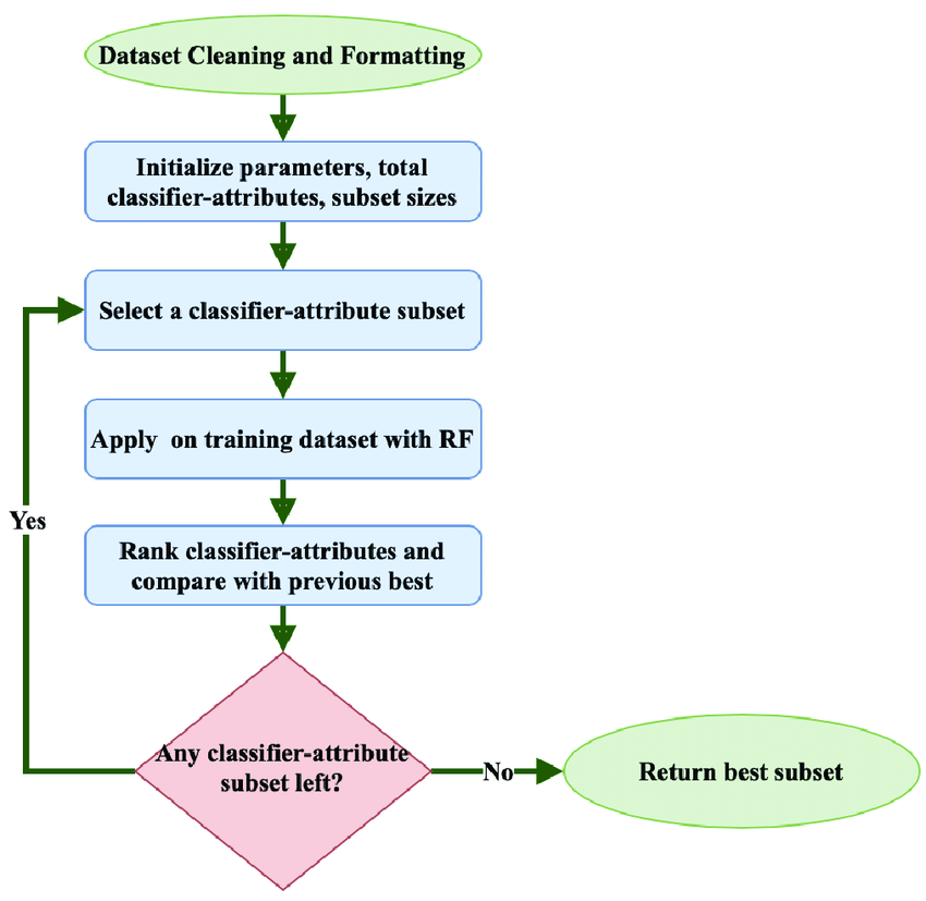
### RFE: Workflow and Advantages
- **Automated Feature Selection**: RFE streamlines the often laborious and error-prone task of feature selection. It integrates directly with many classification and regression models.
- **Feature Ranking and Selection**: In addition to marking a feature for elimination, RFE provides a ranked list of features, helping to establish cut-off points based on business needs or predictive accuracy.
- **Considers Feature Interactions**: By allowing models (such as decision trees) to re-evaluate feature importance after each elimination, RFE can capture intricate relationships between variables.
### Pitfalls and Considerations
- **Model Sensitivity**: RFE might yield different feature sets when applied to different models, calling for prudence in final feature selection.
- **Computational Demands**: Running RFE on extensive feature sets or datasets can be computationally intensive, requiring judicious use on such data.
- **Scalable Solutions**: For large datasets, approaches like **Randomized LASSO** and **Randomized Logistic Regression** provide quicker, albeit approximate, feature rankings.
### Code Example: Recursive Feature Elimination
Here is the Python code:
```python
from sklearn.feature_selection import RFE
from sklearn.linear_model import LogisticRegression
from sklearn.datasets import load_iris
# Load the dataset
data = load_iris()
X, y = data.data, data.target
# Create the RFE model and select top 2 features
rfe_model = RFE(estimator=LogisticRegression(), n_features_to_select=2)
X_rfe = rfe_model.fit_transform(X, y)
# Print the top features
print("Top features after RFE:")
print(X_rfe)
```
#### Explore all 50 answers here 👉 [Devinterview.io - Feature Engineering](https://devinterview.io/questions/machine-learning-and-data-science/feature-engineering-interview-questions)