https://github.com/devinterview-io/graph-data-structure-interview-questions
🟣 Graph Data Structure interview questions and answers to help you prepare for your next data structures and algorithms interview in 2024.
https://github.com/devinterview-io/graph-data-structure-interview-questions
algorithms algorithms-and-data-structures algorithms-and-data-structures-interview-questions algorithms-interview-questions coding-interview-questions data-structures data-structures-and-algorithms data-structures-and-algorithms-interview-questions data-structures-interview-questions graph-data-structure graph-data-structure-interview-questions graph-data-structure-questions graph-data-structure-tech-interview software-architecture-interview software-architecture-interview-questions software-developer-interview software-engineer-interview
Last synced: 4 months ago
JSON representation
🟣 Graph Data Structure interview questions and answers to help you prepare for your next data structures and algorithms interview in 2024.
- Host: GitHub
- URL: https://github.com/devinterview-io/graph-data-structure-interview-questions
- Owner: Devinterview-io
- Created: 2021-01-24T08:14:14.000Z (over 5 years ago)
- Default Branch: main
- Last Pushed: 2024-01-06T19:28:31.000Z (over 2 years ago)
- Last Synced: 2025-03-30T22:16:32.412Z (about 1 year ago)
- Topics: algorithms, algorithms-and-data-structures, algorithms-and-data-structures-interview-questions, algorithms-interview-questions, coding-interview-questions, data-structures, data-structures-and-algorithms, data-structures-and-algorithms-interview-questions, data-structures-interview-questions, graph-data-structure, graph-data-structure-interview-questions, graph-data-structure-questions, graph-data-structure-tech-interview, software-architecture-interview, software-architecture-interview-questions, software-developer-interview, software-engineer-interview
- Homepage: https://devinterview.io/
- Size: 25.4 KB
- Stars: 10
- Watchers: 1
- Forks: 1
- Open Issues: 0
-
Metadata Files:
- Readme: README.md
Awesome Lists containing this project
README
# 50 Essential Graph Data Structure Interview Questions in 2026
#### You can also find all 50 answers here 👉 [Devinterview.io - Graph Data Structure](https://devinterview.io/questions/data-structures-and-algorithms/graph-data-structure-interview-questions)
## 1. What is a _Graph_?
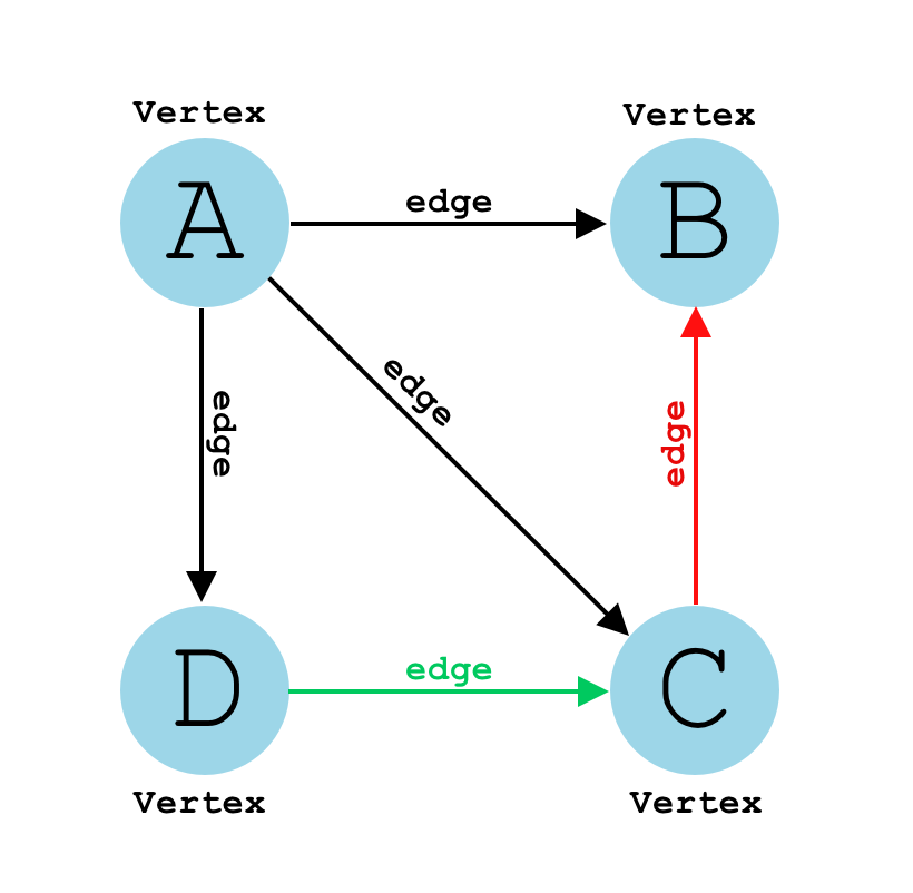
A **graph** is a data structure that represents a collection of interconnected **nodes** through a set of **edges**.
This abstract structure is highly versatile and finds applications in various domains, from social network analysis to computer networking.
### Core Components
A graph consists of two main components:
1. **Nodes**: Also called **vertices**, these are the fundamental units that hold data.
2. **Edges**: These are the connections between nodes, and they can be either **directed** or **undirected**.
### Visual Representation
### Graph Representations
There are several ways to represent graphs in computer memory, with the most common ones being **adjacency matrix**, **adjacency list**, and **edge list**.
#### Adjacency Matrix
In an adjacency matrix, a 2D Boolean array indicates the edges between nodes. A value of `True` at index `[i][j]` means that an edge exists between nodes `i` and `j`.
Here is the Python code:
```python
graph = [
[False, True, True],
[True, False, True],
[True, True, False]
]
```
#### Adjacency List
An adjacency list represents each node as a list, and the indices of the list are the nodes. Each node's list contains the nodes that it is directly connected to.
Here is the Python code:
```python
graph = {
0: [1, 2],
1: [0, 2],
2: [0, 1]
}
```
#### Edge List
An edge list is a simple list of tuples, where each tuple represents an edge between two nodes.
Here is the Python code:
```python
graph = [(0, 1), (0, 2), (1, 2)]
```
## 2. What are some common _Types_ and _Categories_ of _Graphs_?
Graphs serve as **adaptable data structures** for various computational tasks and real-world applications. Let's look at their diverse types.
### Types of Graphs
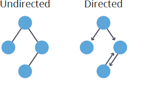
1. **Undirected**: Edges lack direction, allowing free traversal between connected nodes. Mathematically, $(u,v)$ as an edge implies $(v,u)$ as well.
2. **Directed (Digraph)**: Edges have a set direction, restricting traversal accordingly. An edge $(u,v)$ doesn't guarantee $(v,u)$.
#### Weight Considerations
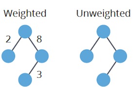
1. **Weighted**: Each edge has a numerical "weight" or "cost."
2. **Unweighted**: All edges are equal in weight, typically considered as 1.
#### Presence of Cycles
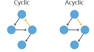
1. **Cyclic**: Contains at least one cycle or closed path.
2. **Acyclic**: Lacks cycles entirely.
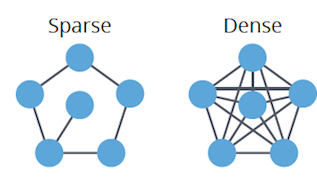
#### Edge Density
1. **Dense**: High edge-to-vertex ratio, nearing the maximum possible connections.
2. **Sparse**: Low edge-to-vertex ratio, closer to the minimum.
#### Connectivity
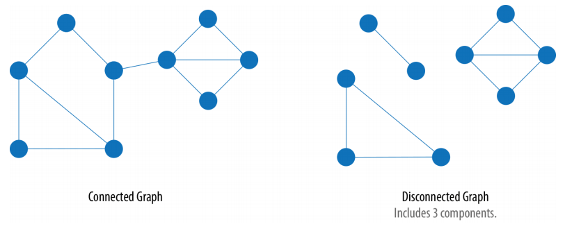
1. **Connected**: Every vertex is reachable from any other vertex.
2. **Disconnected**: Some vertices are unreachable from others.
#### Edge Uniqueness
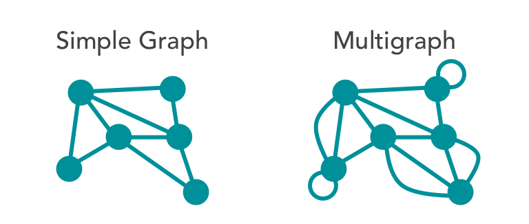
1. **Multigraph**: Allows duplicate edges between vertices.
2. **Simple**: Limits vertices to a single connecting edge.
## 3. What is the difference between a _Tree_ and a _Graph_?
**Graphs** and **trees** are both nonlinear data structures, but there are fundamental distinctions between them.
### Key Distinctions
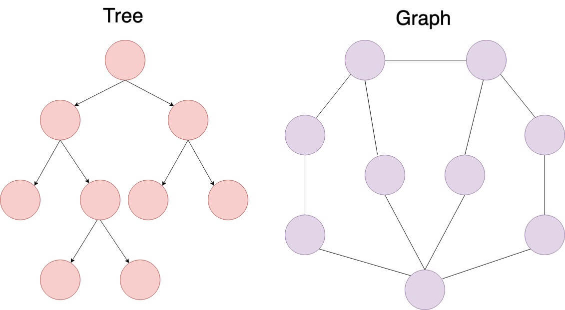
- **Uniqueness**: Trees have a single root, while graphs may not have such a concept.
- **Topology**: Trees are **hierarchical**, while graphs can exhibit various structures.
- **Focus**: Graphs center on relationships between individual nodes, whereas trees emphasize the relationship between nodes and a common root.
### Graphs: Versatile and Unstructured
- **Elements**: Composed of vertices/nodes (denoted as V) and edges (E) representing relationships. Multiple edges and **loops** are possible.
- **Directionality**: Edges can be directed or undirected.
- **Connectivity**: May be **disconnected**, with sets of vertices that aren't reachable from others.
- **Loops**: Can contain cycles.
### Trees: Hierarchical and Organized
- **Elements**: Consist of nodes with parent-child relationships.
- **Directionality**: Edges are strictly parent-to-child.
- **Connectivity**: Every node is accessible from the unique root node.
- **Loops**: Cycles are not allowed.
### Visual Representation
## 4. How can you determine the _Minimum number of edges_ for a graph to remain connected?
To ensure a graph remains **connected**, it must have a minimum number of edges determined by the number of vertices. This is known as the **edge connectivity** of the graph.
### Edge Connectivity Formula
The minimum number of edges required for a graph to remain connected is given by:
$$
\text{{Edge Connectivity}} = \max(\delta(G),1)
$$
Where:
- $\delta(G)$ is the minimum degree of a vertex in $G$.
- The maximum function ensures that the graph remains connected even if all vertices have a degree of 1 or 0.
For example, a graph with a minimum vertex degree of 3 or more requires at least 3 edges to stay connected.
## 5. Define _Euler Path_ and _Euler Circuit_ in the context of graph theory.
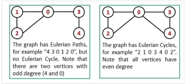
In **graph theory**, an **Euler Path** and an **Euler Circuit** serve as methods to visit all edges (links) exactly once, with the distinction that an Euler Circuit also visits all vertices once.
### Euler Path and Euler Circuit Definitions
A graph has an **Euler Path** if it contains exactly two vertices of odd degree.
A graph has an **Euler Circuit** if every vertex has even degree.
**Degree** specifies the number of edges adjacent to a vertex.
### Key Concepts
- **Starting Vertex**: In an Euler Path, the unique starting and ending vertices are the two with odd degrees.
- **Reachability**: In both Euler Path and Circuit, every edge must be reachable from the starting vertex.
- **Direction-Consistency**: While an Euler Path is directionally open-ended, an Euler Circuit is directionally closed.
### Visual Representation: Euler Path and Circuit
## 6. Compare _Adjacency Lists_ and _Adjacency Matrices_ for graph representation.
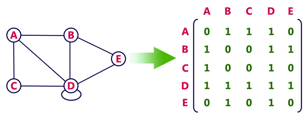
Graphs can be represented in various ways, but **Adjacency Matrix** and **Adjacency List** are the most commonly used data structures. Each method offers distinct advantages and trade-offs, which we'll explore below.
### Space Complexity
- **Adjacency Matrix**: Requires a $N \times N$ matrix, resulting in $O(N^2)$ space complexity.
- **Adjacency List**: Utilizes a list or array for each node's neighbors, leading to $O(N + E)$ space complexity, where $E$ is the number of edges.
### Time Complexity for Edge Look-Up
- **Adjacency Matrix**: Constant time, $O(1)$, as the presence of an edge is directly accessible.
- **Adjacency List**: Up to $O(k)$, where $k$ is the degree of the vertex, as the list of neighbors may need to be traversed.
### Time Complexity for Traversal
- **Adjacency Matrix**: Requires $O(N^2)$ time to iterate through all potential edges.
- **Adjacency List**: Takes $O(N + E)$ time, often faster for sparse graphs.
### Time Complexity for Edge Manipulation
- **Adjacency Matrix**: $O(1)$ for both addition and removal, as it involves updating a single cell.
- **Adjacency List**: $O(k)$ for addition or removal, where $k$ is the degree of the vertex involved.
### Time Complexity for Vertex Manipulation
- **Adjacency Matrix**: $O(N^2)$ as resizing the matrix is needed.
- **Adjacency List**: $O(1)$ as it involves updating a list or array.
### Code Example: Adjacency Matrix & Adjacency List
Here is the Python code:
```python
adj_matrix = [
[0, 1, 1, 0, 0, 0],
[1, 0, 0, 1, 0, 0],
[1, 0, 0, 0, 0, 1],
[0, 1, 0, 0, 1, 1],
[0, 0, 0, 1, 0, 0],
[0, 0, 1, 1, 0, 0]
]
adj_list = [
[1, 2],
[0, 3],
[0, 5],
[1, 4, 5],
[3],
[2, 3]
]
```
## 7. What is an _Incidence Matrix_, and when would you use it?
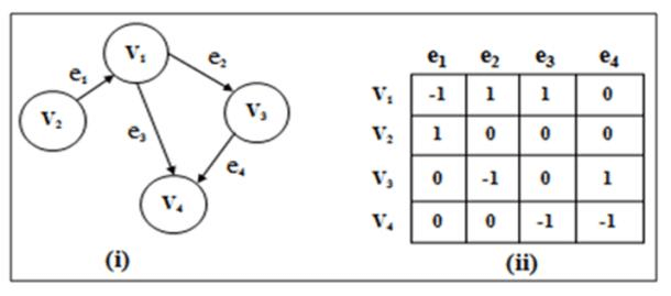
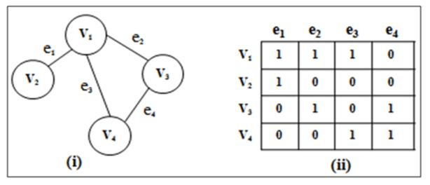
An **incidence matrix** is a binary graph representation that maps vertices to edges. It's especially useful for **directed** and **multigraphs**. The matrix contains $0$s and $1$s, with positions corresponding to "vertex connected to edge" relationships.
### Matrix Structure
- **Columns**: Represent edges
- **Rows**: Represent vertices
- **Cells**: Indicate whether a vertex is connected to an edge
Each unique **row-edge pair** depicts an incidence of a vertex in an edge, relating to the graph's structure differently based on the graph type.
### Example: Incidence Matrix for a Directed Graph
### Example: Incidence Matrix for an Undirected Multigraph
### Applications of Incidence Matrices
- **Algorithm Efficiency**: Certain matrix operations can be faster than graph traversals.
- **Graph Comparisons**: It enables direct graph-to-matrix or matrix-to-matrix comparisons.
- **Database Storage**: A way to represent graphs in databases amongst others.
- **Graph Transformations**: Useful in transformations like line graphs and dual graphs.
## 8. Discuss _Edge List_ as a graph representation and its use cases.
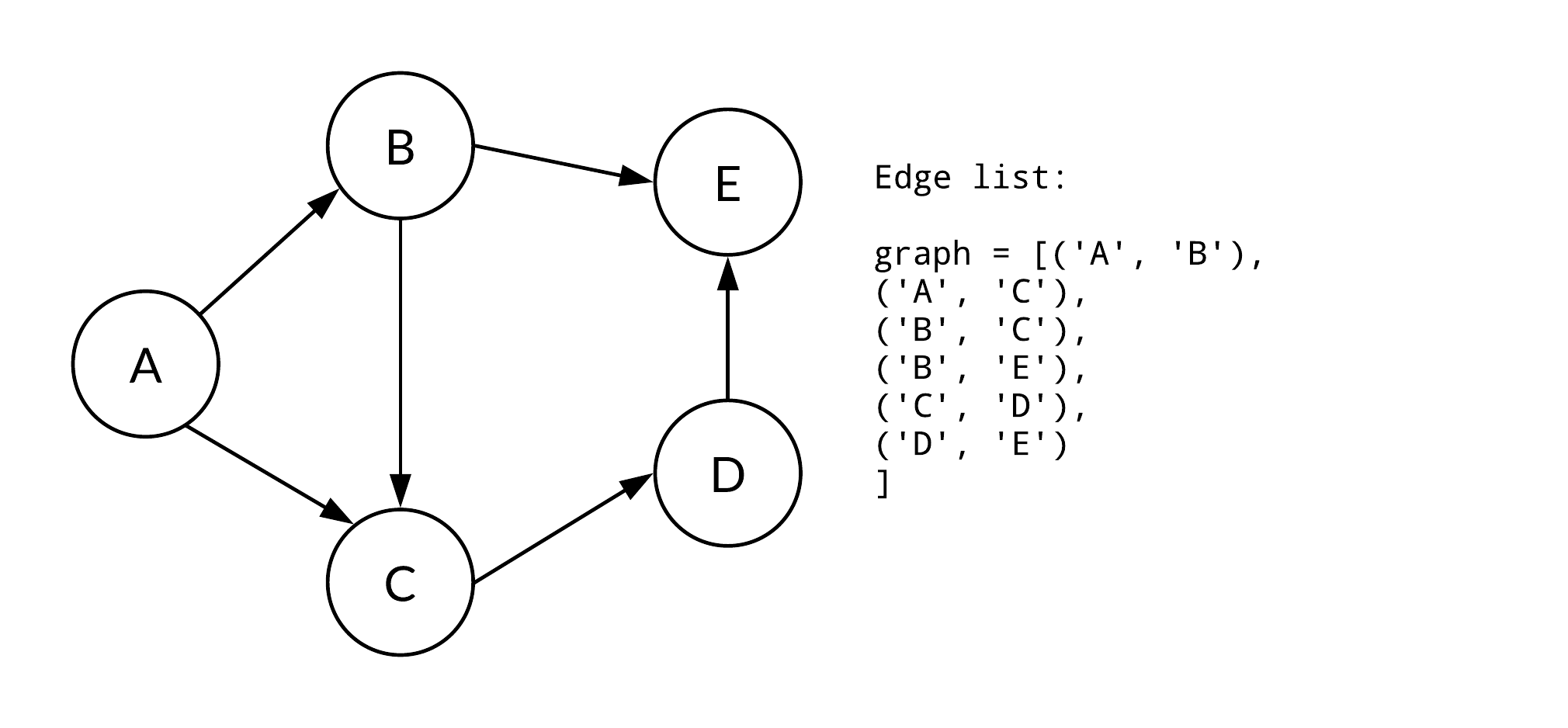
**Edge list** is a straightforward way to represent graphs. It's apt for dense graphs and offers a quick way to query edge information.
### Key Concepts
- **Edge Storage**: The list contains tuples (a, b) to denote an edge between nodes $a$ and $b$.
- **Edge Direction**: The edges can be directed or undirected.
- **Edge Duplicates**: Multiple occurrences signal multigraph. Absence ensures simple graph.
### Visual Example
### Code Example: Edge List
Here is the Python 3 code:
```python
# Example graph
edges = {('A', 'B'), ('A', 'C'), ('B', 'C'), ('C', 'D'), ('B', 'D'), ('D', 'E')}
# Check existence
print(('A', 'B') in edges) # True
print(('B', 'A') in edges) # False
print(('A', 'E') in edges) # False
# Adding an edge
edges.add(('E', 'C'))
# Removing an edge
edges.remove(('D', 'E'))
print(edges) # Updated set: {('A', 'C'), ('B', 'D'), ('C', 'D'), ('A', 'B'), ('E', 'C'), ('B', 'C')}
```
## 9. Explain how to save space while storing a graph using _Compressed Sparse Row_ (CSR).
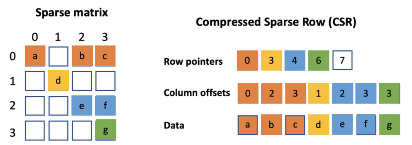
In **Compressed Sparse Row** format, the graph is represented by three linked arrays. This streamlined approach can significantly reduce memory use and is especially beneficial for **sparse graphs**.
Let's go through the data structures and the detailed process.
### Data Structures
1. **Indptr Array (IA)**: A list of indices where each row starts in the `adj_indices` array. It's of length `n_vertices + 1`.
2. **Adjacency Index Array (AA)**: The column indices for each edge based on their position in the `indptr` array.
3. **Edge Data**: The actual edge data. This array's length matches the number of non-zero elements.
### Visual Representation
### Code Example: CSR Graph Representation
Here is the Python code:
```python
indptr = [0, 2, 3, 5, 6, 7, 8]
indices = [2, 4, 0, 1, 3, 4, 2, 3]
data = [1, 2, 3, 4, 5, 6, 7, 8]
# Reading from the CSR Format
for i in range(len(indptr) - 1):
start = indptr[i]
end = indptr[i + 1]
print(f"Vertex {i} is connected to vertices {indices[start:end]} with data {data[start:end]}")
# Writing a CSR Represented Graph
# Vertices 0 to 5, Inclusive.
# 0 -> [2, 3, 4] - Data [3, 5, 7]
# 1 -> [0] - Data [1]
# 2 -> [] - No outgoing edges.
# 3 -> [1] - Data [2]
# 4 -> [3] - Data [4]
# 5 -> [2] - Data [6]
# Code to populate:
# indptr = [0, 3, 4, 4, 5, 6, 7]
# indices = [2, 3, 4, 0, 1, 3, 2]
# data = [3, 5, 7, 1, 2, 4, 6]
```
## 10. Explain the _Breadth-First Search_ (BFS) traversing method.
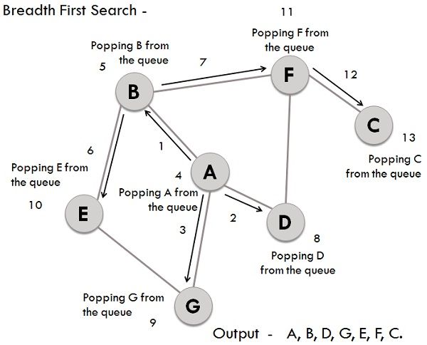
**Breadth-First Search** (BFS) is a graph traversal technique that systematically explores a graph level by level. It uses a **queue** to keep track of nodes to visit next and a list to record visited nodes, avoiding redundancy.
### Key Components
- **Queue**: Maintains nodes in line for exploration.
- **Visited List**: Records nodes that have already been explored.
### Algorithm Steps
1. **Initialize**: Choose a starting node, mark it as visited, and enqueue it.
2. **Explore**: Keep iterating as long as the queue is not empty. In each iteration, dequeue a node, visit it, and enqueue its unexplored neighbors.
3. **Terminate**: Stop when the queue is empty.
### Visual Representation
### Complexity Analysis
- **Time Complexity**: $O(V + E)$ where $V$ is the number of vertices in the graph and $E$ is the number of edges. This is because each vertex and each edge will be explored only once.
- **Space Complexity**: $O(V)$ since, in the worst case, all of the vertices can be inside the queue.
### Code Example: Breadth-First Search
Here is the Python code:
```python
from collections import deque
def bfs(graph, start):
visited = set()
queue = deque([start])
while queue:
vertex = queue.popleft()
if vertex not in visited:
print(vertex, end=' ')
visited.add(vertex)
queue.extend(neighbor for neighbor in graph[vertex] if neighbor not in visited)
# Sample graph representation using adjacency sets
graph = {
'A': {'B', 'D', 'G'},
'B': {'A', 'E', 'F'},
'C': {'F'},
'D': {'A', 'F'},
'E': {'B'},
'F': {'B', 'C', 'D'},
'G': {'A'}
}
# Execute BFS starting from 'A'
bfs(graph, 'A')
# Expected Output: 'A B D G E F C'
```
## 11. Explain the _Depth-First Search_ (DFS) algorithm.
**Depth-First Search** (DFS) is a graph traversal algorithm that's simpler and **often faster** than its breadth-first counterpart (BFS). While it **might not explore all vertices**, DFS is still fundamental to numerous graph algorithms.
### Algorithm Steps
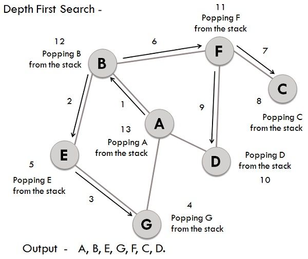
1. **Initialize**: Select a starting vertex, mark it as visited, and put it on a stack.
2. **Loop**: Until the stack is empty, do the following:
- Remove the top vertex from the stack.
- Explore its unvisited neighbors and add them to the stack.
3. **Finish**: When the stack is empty, the algorithm ends, and all reachable vertices are visited.
### Visual Representation
### Code Example: Depth-First Search
Here is the Python code:
```python
def dfs(graph, start):
visited = set()
stack = [start]
while stack:
vertex = stack.pop()
if vertex not in visited:
visited.add(vertex)
stack.extend(neighbor for neighbor in graph[vertex] if neighbor not in visited)
return visited
# Example graph
graph = {
'A': {'B', 'G'},
'B': {'A', 'E', 'F'},
'G': {'A'},
'E': {'B', 'G'},
'F': {'B', 'C', 'D'},
'C': {'F'},
'D': {'F'}
}
print(dfs(graph, 'A')) # Output: {'A', 'B', 'C', 'D', 'E', 'F', 'G'}
```
## 12. What are the key differences between _BFS_ and _DFS_?
**BFS** and **DFS** are both essential graph traversal algorithms with distinct characteristics in strategy, memory requirements, and use-cases.
### Core Differences
1. **Search Strategy**: BFS moves level-by-level, while DFS goes deep into each branch before backtracking.
2. **Data Structures**: BFS uses a Queue, whereas DFS uses a Stack or recursion.
3. **Space Complexity**: BFS requires more memory as it may need to store an entire level ($O(|V|)$), whereas DFS usually uses less ($O(\log n)$ on average).
4. **Optimality**: BFS guarantees the shortest path; DFS does not.
### Visual Representation
#### BFS
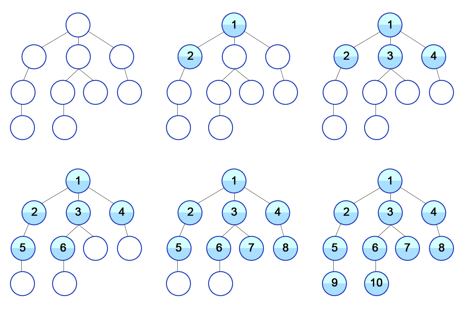
#### DFS

### Code Example: BFS & DFS
Here is the Python code:
```python
# BFS
def bfs(graph, start):
visited = set()
queue = [start]
while queue:
node = queue.pop(0)
if node not in visited:
visited.add(node)
queue.extend(graph[node] - visited)
# DFS
def dfs(graph, start, visited=None):
if visited is None:
visited = set()
visited.add(start)
for next_node in graph[start] - visited:
dfs(graph, next_node, visited)
```
## 13. Implement a method to check if there is a _Path between two vertices_ in a graph.
### Problem Statement
Given an **undirected** graph, the task is to determine whether or not there is a **path** between two specified vertices.
### Solution
The problem can be solved using **Depth-First Search (DFS)**.
#### Algorithm Steps
1. Start from the source vertex.
2. For each adjacent vertex, if not visited, recursively perform DFS.
3. If the destination vertex is found, return `True`. Otherwise, backtrack and explore other paths.
#### Complexity Analysis
- **Time Complexity**: $O(V + E)$
$V$ is the number of vertices, and $E$ is the number of edges.
- **Space Complexity**: $O(V)$
For the stack used in recursive DFS calls.
#### Implementation
Here is the Python code:
```python
from collections import defaultdict
class Graph:
def __init__(self):
self.graph = defaultdict(list)
def add_edge(self, u, v):
self.graph[u].append(v)
self.graph[v].append(u)
def is_reachable(self, src, dest, visited):
visited[src] = True
if src == dest:
return True
for neighbor in self.graph[src]:
if not visited[neighbor]:
if self.is_reachable(neighbor, dest, visited):
return True
return False
def has_path(self, src, dest):
visited = defaultdict(bool)
return self.is_reachable(src, dest, visited)
# Usage
g = Graph()
g.add_edge(0, 1)
g.add_edge(0, 2)
g.add_edge(1, 2)
g.add_edge(2, 3)
g.add_edge(3, 3)
source, destination = 0, 3
print(f"There is a path between {source} and {destination}: {g.has_path(source, destination)}")
```
## 14. Solve the problem of printing all _Paths from a source to destination_ in a Directed Graph with BFS or DFS.
### Problem Statement
Given a **directed graph** and two vertices $src$ and $dest$, the objective is to **print all paths** from $src$ to $dest$.
### Solution
1. **Recursive Depth-First Search (DFS)** Algorithm in Graphs: DFS is used because it can identify all the paths in a graph from source to destination. This is done by employing a **backtracking mechanism** to ensure that all unique paths are found.
2. To deal with **cycles**, a list of visited nodes is crucial. By utilizing this list, the algorithm can avoid revisiting and getting stuck in an infinite loop.
#### Complexity Analysis
- **Time Complexity**: $O(V + E)$
- $V$ is the number of vertices and $E$ is the number of edges.
- We're essentially visiting every node and edge once.
- **Space Complexity**: $O(V)$
- In the worst-case scenario, the entire graph can be visited, which would require space proportional to the number of vertices.
#### Implementation
Here is the Python code:
```python
# Python program to print all paths from a source to destination in a directed graph
from collections import defaultdict
# A class to represent a graph
class Graph:
def __init__(self, vertices):
# No. of vertices
self.V = vertices
# default dictionary to store graph
self.graph = defaultdict(list)
def addEdge(self, u, v):
self.graph[u].append(v)
def printAllPathsUtil(self, u, d, visited, path):
# Mark the current node as visited and store in path
visited[u] = True
path.append(u)
# If current vertex is same as destination, then print current path
if u == d:
print(path)
else:
# If current vertex is not destination
# Recur for all the vertices adjacent to this vertex
for i in self.graph[u]:
if not visited[i]:
self.printAllPathsUtil(i, d, visited, path)
# Remove current vertex from path and mark it as unvisited
path.pop()
visited[u] = False
# Prints all paths from 's' to 'd'
def printAllPaths(self, s, d):
# Mark all the vertices as not visited
visited = [False] * (self.V)
# Create an array to store paths
path = []
path.append(s)
# Call the recursive helper function to print all paths
self.printAllPathsUtil(s, d, visited, path)
# Create a graph given in the above diagram
g = Graph(4)
g.addEdge(0, 1)
g.addEdge(0, 2)
g.addEdge(0, 3)
g.addEdge(2, 0)
g.addEdge(2, 1)
g.addEdge(1, 3)
s = 2 ; d = 3
print("Following are all different paths from %d to %d :" %(s, d))
g.printAllPaths(s, d)
```
## 15. What is a _Bipartite Graph_? How to detect one?
A **bipartite graph** is one where the vertices can be divided into two distinct sets, $U$ and $V$, such that every edge connects a vertex from $U$ to one in $V$. The graph is denoted as $G = (U, V, E)$, where $E$ represents the set of edges.

### Detecting a Bipartite Graph
You can check if a graph is bipartite using several methods:
#### Breadth-First Search (BFS)
BFS is often used for this purpose. The algorithm colors vertices alternately so that no adjacent vertices have the same color.
#### Code Example: Bipartite Graph using BFS
Here is the Python code:
```python
from collections import deque
def is_bipartite_bfs(graph, start_node):
visited = {node: False for node in graph}
color = {node: None for node in graph}
color[start_node] = 1
queue = deque([start_node])
while queue:
current_node = queue.popleft()
visited[current_node] = True
for neighbor in graph[current_node]:
if not visited[neighbor]:
queue.append(neighbor)
color[neighbor] = 1 - color[current_node]
elif color[neighbor] == color[current_node]:
return False
return True
# Example
graph = {'A': ['B', 'C'], 'B': ['A', 'C'], 'C': ['A', 'B', 'D'], 'D': ['C']}
print(is_bipartite_bfs(graph, 'A')) # Output: True
```
#### Cycle Detection
A graph is not bipartite if it contains an odd cycle. Algorithms like **DFS** or **Floyd's cycle-detection** algorithm can help identify such cycles.
#### Explore all 50 answers here 👉 [Devinterview.io - Graph Data Structure](https://devinterview.io/questions/data-structures-and-algorithms/graph-data-structure-interview-questions)
