https://github.com/devinterview-io/neural-networks-interview-questions
🟣 Neural Networks interview questions and answers to help you prepare for your next machine learning and data science interview in 2024.
https://github.com/devinterview-io/neural-networks-interview-questions
ai-interview-questions coding-interview-questions coding-interviews data-science data-science-interview data-science-interview-questions data-scientist-interview interview-practice interview-preparation machine-learning machine-learning-and-data-science machine-learning-interview machine-learning-interview-questions neural-networks neural-networks-interview-questions neural-networks-questions neural-networks-tech-interview software-engineer-interview technical-interview-questions
Last synced: 6 months ago
JSON representation
🟣 Neural Networks interview questions and answers to help you prepare for your next machine learning and data science interview in 2024.
- Host: GitHub
- URL: https://github.com/devinterview-io/neural-networks-interview-questions
- Owner: Devinterview-io
- Created: 2024-01-08T17:03:13.000Z (over 2 years ago)
- Default Branch: main
- Last Pushed: 2024-01-08T17:12:40.000Z (over 2 years ago)
- Last Synced: 2025-02-06T02:49:00.147Z (over 1 year ago)
- Topics: ai-interview-questions, coding-interview-questions, coding-interviews, data-science, data-science-interview, data-science-interview-questions, data-scientist-interview, interview-practice, interview-preparation, machine-learning, machine-learning-and-data-science, machine-learning-interview, machine-learning-interview-questions, neural-networks, neural-networks-interview-questions, neural-networks-questions, neural-networks-tech-interview, software-engineer-interview, technical-interview-questions
- Size: 17.6 KB
- Stars: 6
- Watchers: 1
- Forks: 1
- Open Issues: 0
-
Metadata Files:
- Readme: README.md
Awesome Lists containing this project
README
# 95 Common Neural Networks Interview Questions in 2026

#### You can also find all 95 answers here 👉 [Devinterview.io - Neural Networks](https://devinterview.io/questions/machine-learning-and-data-science/neural-networks-interview-questions)
## 1. What is a _neural network_, and how does it resemble _human brain functionality_?
A **neural network** is a computational model inspired by the structure and function of the human brain. It is increasingly used in a wide range of applications, particularly in **Machine Learning** tasks and **pattern recognition**.
### Structural Parallels
- **Neuron**: The fundamental computational unit, akin to a single brain cell. It processes incoming signals, modifies them, and transmits the result.
- **Synapse**: The connection through which neurons communicate. In neural networks, synapses represent weights that modulate information flow from one neuron to the next.
- **Layers**: Organized sets of neurons in the network, each with a specific role in processing the input. Neurons in adjacent layers are interconnected, mimicking the interconnectedness of neurons in the brain.
### Key Functions of Neurons and Synthetic Counterparts
#### Real Neurons
- **Excitation/Inhibition**: Neurons become more or less likely to fire, altering signal transmission.
- **Thresholding**: Neurons fire only after receiving a certain level of stimulus.
- **Summation**: Neurons integrate incoming signals before deciding whether to fire.
#### Artificial Neurons
In a simplified binary form, they perform excitation by "firing" (i.e., being active) or inhibition by remaining "silent".
In a more complex form like the Sigmoid function, neurons are a continuous version of their binary counterparts.
### Learning Paradigms
#### Real Neurons
- **Adaptive**: Through a process called synaptic plasticity, synapses can be strengthened or weakened in response to neural activity. This mechanism underpins learning, memory, and cognitive functions.
- **Feedback Mechanisms**: Signals, such as hormones or neurotransmitters, provide feedback about the consequences of neural activity, influencing future behavior.
#### Artificial Neurons
- **Learning Algorithms**: They draw from several biological theories, like Hebbian learning, and computational principles, ensuring the network improves its performance on tasks.
- **Feedback from Preceding Layers**: Weight updates in the network are the result of backpropagating errors from the output layer to the input layer. This is the artificial equivalent of understanding the consequences of decisions to guide future ones.
### Code Example: Sigmoid Activation Function
Here is the Python code:
```python
# Sigmoid Function
def sigmoid(x):
return 1 / (1 + np.exp(-x))
```
## 2. Elaborate on the structure of a basic _artificial neuron_.
The **Artificial Neuron** serves as the fundamental building block of artificial neural networks, and from it, several artificial intelligence paradigms have emerged.
### Structure of an Artificial Neuron
At its core, the artificial neuron is a simplified model of a biological neuron. The **input signals**, $x_1, x_2, \ldots, x_n$, are received through **dendrites**, weighted in the **synaptic terminals** of the neuron, and passed through an **activation function** to produce the **output**, $y$.
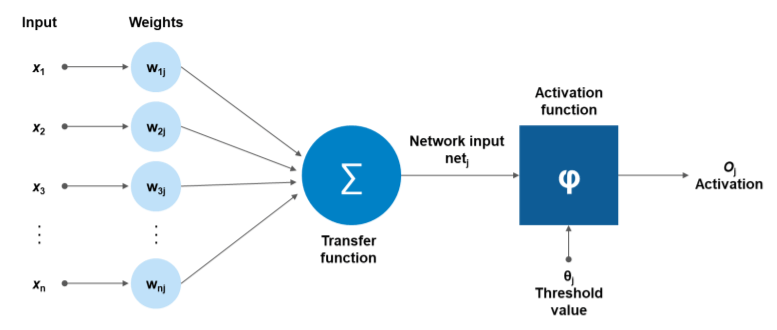
Mathematically, this is represented as:
$$
y = f(\sum_{i=1}^{n} w_i \cdot x_i + b)
$$
Where:
- $x_i$: Input signals
- $w_i$: Corresponding synaptic weights
- $b$: Bias term
- $f()$: Activation function
### Components of an Artificial Neuron
1. **Inputs**: Numeric values that the neuron processes. Each input is weighted by a synaptic weight.
2. **Synaptic Weights**: Multipliers that control the impact of inputs. They can enhance or diminish the input's influence.
3. **Aggregator**: Neurons in the previous layer are computationally aggregated. In a basic neuron, this requires summing the products of inputs and their respective weights.
Let $z$ represent the weighted sum of inputs:
$$
z = \sum_{i=1}^{n} w_i \cdot x_i + b
$$
Where:
- $w_i$: Synaptic weight for the $i$th input.
- $x_i$: $i$th input.
- $b$: Bias term, which helps the neuron to "fire" by shifting the activation value.
4. **Activation Function**: The aggregated value $z$ is typically passed through a non-linear activation function, $\sigma(z)$, which introduces non-linearities in the neuron's output.
5. **Output**: The final, processed value from the neuron. This could be the output of the neuron itself, or it could be passed on to other neurons in subsequent layers.
#### Activation Functions
Common activation functions include the **Sigmoid**, **Hyperbolic Tangent (Tanh)**, **Rectified Linear Unit (ReLU)**, and **Softmax**.
### Code Example: Basic Artificial Neuron
Here is the Python code:
```python
import numpy as np
class ArtificialNeuron:
def __init__(self, num_inputs):
# Initialize weights and bias
self.weights = np.random.rand(num_inputs)
self.bias = np.random.rand()
def sigmoid(self, z):
return 1 / (1 + np.exp(-z))
def activate(self, inputs):
# Weighted sum
z = np.dot(inputs, self.weights) + self.bias
# Apply activation function
return self.sigmoid(z)
# Example usage
neuron = ArtificialNeuron(3) # 3 inputs
print(neuron.activate(np.array([0.5, 0.3, 0.8])))
```
## 3. Describe the architecture of a _multi-layer perceptron (MLP)_.
The **Multi-Layer Perceptron** (MLP) is a foundational and versatile neural network model. It consists of **layers** of **neurons**, each connected to the next layer, and leverages non-linear activation functions to model complex relationships in the data.
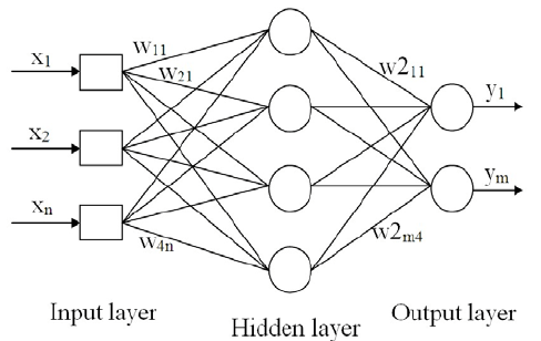
### Key Components
1. **Input Layer**: Contains nodes that represent the input features. These nodes don't perform any computation and directly pass their values to the next layer.
2. **Hidden Layers**: Consist of neurons that transform the inputs using weighted sums and activation functions. The number of hidden layers and their nodes determine the model's **architecture**.
3. **Output Layer**: Generates the final predictions or class probabilities.
4. **Weights and Biases**: Parameters that are learned during training and control the strength and direction of the neuron connections.
5. **Activation Functions**: Non-linear functions applied to the weighted sums of the neuron inputs. They introduce non-linearity and enhance the model's expressive power.
### Activation Functions
Several activation functions are commonly used, such as:
- **Sigmoid**: Smoothly maps inputs to a range between 0 and 1. Useful for binary classification and tasks where output probabilities are desired.
```python
import numpy as np
def sigmoid(x):
return 1 / (1 + np.exp(-x))
```
- **ReLU (Rectified Linear Unit)**: Sets negative values to zero and preserves positive values. Popular due to its computational efficiency and effectiveness in many tasks.
```python
def relu(x):
return np.maximum(0, x)
```
## 4. How does _feedforward neural network_ differ from _recurrent neural networks (RNNs)_?
The **feedforward neural network** and **recurrent neural network** (RNN) have distinct architectures and are used for different tasks and data types.
### Feedforward Neural Network (FFNN)
In a **feedforward neural network**, data travels in one direction: from input nodes through hidden nodes to output nodes.
### Recurrent Neural Network (RNN)
In contrast, **RNNs** have feedback loops allowing information to persist. This enables them to process sequences of inputs, making them suitable for tasks like time-series forecasting or natural language processing (NLP).
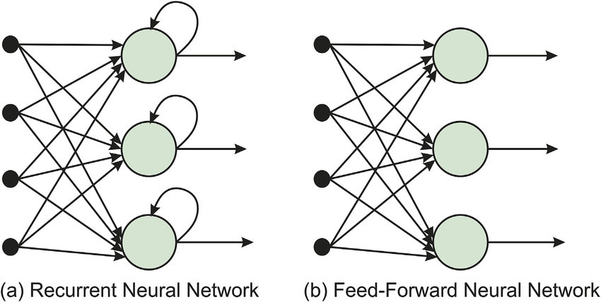
### Key Distinctions
#### Data Processing
- **Feedforward**: Each data point is processed independently of others. This makes FFNNs suitable for static datasets and single-sample predictions.
- **RNN**: Data sequences, like sentences or time series, are processed sequentially, where present inputs depend on past ones.
#### Information Flow
- **Feedforward**: One-directional. The network's output doesn't influence its input.
- **RNN**: Bi-directional due to feedback loops. Past experiences influence present and future computations.
#### Memory
- **Feedforward**: Stateless, i.e., no memory of previous inputs.
- **RNN**: Possesses memory because of its feedback loops. However, RNNs can face long-term dependency challenges where crucial historic information might be diluted or forgotten over time. This has led to the development of different RNN architectures and also alternatives such as Long Short-Term Memory (LSTM) and Gated Recurrent Unit (GRU) networks, which aim to address this limitation by having selective, long-lasting memory.
#### Time Sensitivity
- **Feedforward**: Instantaneous. The model generates outputs instantaneously based solely on the present input data point.
- **RNN**: Time-sensitive. Past inputs influence the current state, making RNNs suitable for dynamic, time-varying data.
### Practical Examples
- **FFNN**: Image or text classification tasks where each input is independent.
- **RNN**: Tasks like speech recognition, language translation, or stock prediction that involve sequences or time-series data.
## 5. What is _backpropagation_, and why is it important in _neural networks_?
**Backpropagation** is a critical algorithm in neural network training, allowing for the **adjustment of weights and biases** based on prediction errors.
### Core Components
1. **Forward Pass**: Neurons in each layer apply an activation function to the weighted sum of inputs.
$$
a^{[l]} = g^{[l]}(z^{[l]}) \quad \text{where}~ z^{[l]} = W^{[l]}a^{[l-1]} + b^{[l]}
$$
2. **Error Computation**: Using a **loss function**, the network measures the deviation of its predictions from the targets.
$$
\mathcal{L} = \frac{1}{m} \sum_{i=1}^{m} L(y_i, \hat{y}_i)
$$
3. **Backward Pass**: The calculated error is propagated backward through the layers to determine how each neuron contributed to this error.
$$
\delta^{[l]} = \frac{\partial \mathcal{L}}{\partial z^{[l]}} = g^{[l]\prime} (z^{[l]}) \odot \left({W^{[l+1]}}^T \delta^{[l+1]}\right) \quad l=L-1, L-2, \ldots, 1
$$
4. **Parameter Update**: Using the calculated error, the algorithm computes the gradient of the loss function with respect to weights and biases.
$$
\frac{\partial \mathcal{L}} {\partial W_{ij}^{[l]}} = a_i^{[l-1]} \delta_j^{[l]} \quad \text{and} \quad \frac{\partial \mathcal{L}} {\partial b_j^{[l]}} = \delta_j^{[l]}
$$
This gradient information is then used in an optimizer such as Stochastic Gradient Descent to update model parameters.
### Key Advantages
- **Efficiency**: Calculating the weights' gradient using backpropagation is often faster than alternative methods like the permutation approach.
- **Consistency**: The algorithm ensures that weight updates move the model in a direction that reduces prediction error.
- **Adaptability**: Backpropagation is adaptable to various network architectures and can handle complex, high-dimensional datasets.
### Backpropagation Shortcomings
- **Vanishing and Exploding Gradient**: Gradients in early layers can become extremely small or large, leading to slow convergence or issues with numerical precision.
- **Local Minima**: Although modern neural networks are less prone to getting stuck in local minima, it's still a possibility that can affect convergence.
- **Dependence on Proper Architectural Choice**: The effectiveness of backpropagation can be affected by the model's architecture, requiring careful design.
#### Addressing Shortcomings
- **Activation Functions**: Using non-linear activation functions like ReLU helps prevent vanishing gradients.
- **Batch Normalization**: Normalizing data between layers can mitigate gradient problems.
- **Weight Initialization**: Techniques such as 'Xavier' or 'He' initialization can enhance gradient flow.
- **Gradient Clipping**: Constraining the gradient magnitude can prevent exploding gradients.
### Code Example: Backpropagation
Here is the Python code:
```python
def forward_pass(x, W, b):
z = np.dot(W, x) + b
a = sigmoid(z) # Assuming a sigmoid activation function for hidden layers
return a, z
def compute_cost(AL, Y):
return -np.mean(Y * np.log(AL) + (1 - Y) * np.log(1 - AL))
def backward_pass(x, y, a, z, W, b):
m = x.shape[1]
delta = AL - Y # Derivative of the loss function w.r.t. the activation of the last layer
dW = (1 / m) * np.dot(delta, a.T)
db = (1 / m) * np.sum(delta)
return dW, db
def update_parameters(W, b, dW, db, learning_rate):
W -= learning_rate * dW
b -= learning_rate * db
return W, b
# Training loop
for i in range(num_iterations):
AL, cache = forward_pass(X, W, b)
cost = compute_cost(AL, Y)
dW, db = backward_pass(X, Y, AL, cache, W, b)
W, b = update_parameters(W, b, dW, db, learning_rate)
```
## 6. Explain the role of an _activation function_. Give examples of some common _activation functions_.
An **activation function** essentially decides the level of activation that should be passed on to the next layer, or to the output. This is done through a nonlinear transformation that introduces crucial characteristics to the neural network.
### Key Benefits of Activation Functions
- **Non-Linearity**: Allows neural networks to model complex, non-linear relationships in data.
- Basic Activation Functions are classified into 3 types:
- **Binary Threshold**: These are either activated or not.
- **Linear**: Output is directly proportional to input.
- **Non-linear**: Variety of functions provide continuous, non-linear transformations.
### Common Activation Functions
- **Binary Step**: The output is binary in nature, being either 0 or 1. This function is not often used.
$$
f(x) = \begin{cases}
0 & \text{if}\ x < 0, \\
1 & \text{if}\ x \geq 0.
\end{cases}
$$
- **Linear**: It produces a linear relationship between the input and output. However, as each layer in the neural network can be made equivalent to a single linear layer, linear functions turn out to be of limited use in building deep models.
- **Rectified Linear Unit (ReLU)**: It activates when the input is positive.
$$
f(x) = \max(0, x).
$$
- **Sigmoid**: Squishes real-valued numbers to the range (0, 1). It's often used in binary classification problems because it can be interpreted as a probability.
$$
f(x) = \frac{1}{1 + e^{-x}}.
$$
- **Hyperbolic Tangent**: Similar to the Sigmoid but squishes values to the range (-1, 1).
$$
f(x) = \tanh(x).
$$
- **Leaky ReLU**: An improvement over ReLU that allows a small gradient when the input is negative.
$$
f(x) = \begin{cases}
x & \text{if}\ x > 0\\
0.01x & \text{otherwise}
\end{cases}.
$$
- **Swish**: Combines qualities of ReLU and Sigmoid, benefitting from the best of both worlds.
$$
f(x) = \frac{x}{1 + e^{-x}}.
$$
- **Softmax**: Converts a real-valued vector to a probability distribution.
$$
f(x_i) = \frac{e^{x_i}}{\sum_{j=1}^N e^{x_j}}.
$$
## 7. Describe the concept of _deep learning_ in relation to _neural networks_.
**Deep learning** is a specialized form of **neural network** modeling that's designed to recognize intricate patterns in data. It's especially effective in uncovering **hidden structures** within tasks such as image and speech recognition. The foundation of deep learning lies in its ability to automate feature engineering, reducing the burden on human experts.
### Feature Engineering vs Feature Learning
Traditional machine learning workflows heavily rely on feature engineering. This process necessitates substantial **domain expertise** to not only select relevant features but also engineer them in a way that serves the model best.
In contrast, deep learning employs deep neural networks that serve as **feature extractors**. Each layer of the network progressively refines inputs, aiming to construct abstract, higher-level features. This is known as **feature learning**.
### Deep Learning for Unstructured Data
Deep learning systems are particularly adept at handling unstructured data, which lacks a straightforward data model or does not conform to tabular forma, such as **audio, text, and images**.
For example, a regular image might contain hundreds of thousands of pixels, which act as individual features in traditional machine learning. But deep learning models are designed to **process the raw pixel data directly**, enabling them to decode complex visual features hierarchically.
### Challenges of Deep Learning
Though powerful, deep learning demands substantial computational resources, often requiring dedicated hardware such as GPUs or TPUs. Moreover, as the number of model parameters, layers, and complexity increase, so does the potential for overfitting and the need for expansive datasets.
Furthermore, deep learning models often operate as "black boxes" from an interpretability standpoint, making it tough to discern how they make decisions.
### Singular Model Architecture: Deep Learning
Contrary to traditional machine learning techniques, which frequently use various algorithms (logistic regression, decision trees, etc.), deep learning systems typically deploy **singular model architectures**—such as Convolutional Neural Networks (CNNs) for image-related tasks and Recurrent Neural Networks (RNNs) for sequence-oriented problems.
The deep learning models experience iterative adjustments via backpropagation—this **tuning process** can take considerable computing resources and time but often delivers superior results.
## 8. What’s the difference between _fully connected_ and _convolutional layers_ in a network?
Both fully connected (FC) layers and convolutional layers are **key components** of many neural network architectures, particularly Convolutional Neural Networks (CNNs) and fully connected multilayer perceptrons (MLPs).
### Purpose
- **Fully Connected (FC)** layers: Each neuron in a FC layer is connected to every neuron in the preceding layer, suitable for models like MLPs that focus on global patterns.
- **Convolutional** layers: These layers are particularly well-suited for extracting local features from spatial data, like images or sentences, and maintaining a "sense of locality." The neurons in a convolutional layer will only be connected to nearby pixels or words.
### Memory Conservation
The main limitation of **fully connected** layers in a CNN is that they can be computationally and memory intensive, especially when dealing with high-dimensional inputs, such as high-resolution images.
On the other hand, **convolutional** and **pooling** layers, often used together in a CNN, reduce the need for memory through parameter sharing and spatial pooling operations.
### Parameter Sharing
Convolutional layers are designed to take advantage of the assumption that nearby regions in the input data are likely to possess similar features or information. This assumption, known as "spatial locality," is embedded in the concept of **parameter sharing**.
- **No Parameter Sharing**: In a FC layer, each neuron is associated with its own unique set of weights, and there is no sharing between neurons in the same layer.
- **Parameter Sharing in Convolutional Layers**: Here, a small subset of neurons (determined by the convolutional kernel size) share the same set of weights. This sharing ensures that the same pattern is detected in different spatial locations, reducing the number of parameters required and enhancing generalization.
### Feature Extraction on Spatial Data
For spatial data, such as images, the distinct operations focusing on **feature extraction** are characteristic of convolutional layers.
- **Local Field Move and Feature Extraction**: Convolutions involve a small receptive field that moves over the input image. At each position, the convolution operation extracts local features, enabling the network to weigh the significance of various features locally, contributing to tasks like edge or texture detection in images.
- **Global Coherence for Decision Making**: The resulting feature maps from convolutional layers often contain valuable local information, and each element in a feature map corresponds to a locally weighted sum in the input. Combining these local features using subsequent layers, typically involving both convolutional and pooling operations, allows the network to make global decisions based on the coherent understanding of the entire input.
On the other hand, fully connected layers are designed for **global data processing**, where each neuron is responsible for considering the entire set of features from the preceding layer.
### Built-In Regularization
Due to their smaller number of parameters and the concept of parameter sharing, convolutional layers naturally provide a form of regularization, helping to prevent overfitting, especially when the amount of labeled data is limited.
### Concept of Locality
- **Local Information Processing**: Convolutional layers process information in a localized manner using the concept of a receptive field, which defines the region of input space that influences the computation at a particular position.
- **Global Integration Through Hierarchical Layers**: After consecutive convolutions and pooling operations, the network enhances local-to-global mappings, allowing the final fully connected layers to make class distinctions based on a global understanding of the input.
### Dimensionality Handling
Different neural network layer types handle input and output dimensions differently:
- **Fully Connected Layers**: Each neuron produces a scalar output, resulting in a single vector, thereby introducing a requirement for the flattening of multidimensional inputs.
- **Convolutional Layers**: By using multidimensional convolutional filters, such layers can work directly with spatial input. The notion of local connectivity enables operations that maintain the initial spatial organization of the input.
### Core Building Blocks
- **Fully Connected Layers**: These are the most straightforward network layers, comprising a weighted sum followed by an activation function.
$$
z = \sum_i^N (w_i \cdot x_i) + b
$$
for neuron $i$, output $z$, input $x_i$, weight $w_i$, and bias $b$.
- **Convolutional Layers**: They perform a convolutional operation, followed by a bias addition and an activation function.
$$
z = \sigma (\sum_{m,n} (w_{m,n} \ast x_{m,n}) + b)
$$
where $m, n$ refers to coordinates within the filter and $\ast$ signifies the convolution operation.
### Versatile Architectures
While **fully connected** layers work consistently well for tasks where data is not spatial or sequential (e.g., classic feedforward tasks), **convolutional** layers are particularly effective for handling structured data, such as images, videos, and text, due to their principles of **local connectivity** and **shared weights**. They are the backbone of many computer vision and natural language processing tasks.
### Optimization Considerations
- **Fully Connected Layers**: These typically need a large number of parameters. A common practice is to use techniques like dropout to prevent overfitting, especially if the training data is limited.
- **Convolutional Layers**: Parameter sharing reduces the number of parameters, naturally providing a built-in form of regularization. However, additional measures might still be necessary in some cases.
## 9. What is a _vanishing gradient problem_? How does it affect _training_?
The **vanishing gradient problem** arises during training in deep neural networks. It's characterized by **diminishing gradients**, particularly in early layers of deep networks. Such gradients indicate to the network how to update its parameters for better performance. Their diminishment can **hamper learning** by causing these early layers to learn slowly or not at all.
In effect, the network fails to capture the **rich hierarchical representations** that are foundational to deep learning's effectiveness.
### Causes of Vanishing Gradients
Several factors can lead to this problem, including network architecture and training data characteristics.
- **Activation Functions**: Sigmoid and to a lesser extent, tanh, have saturated regions where gradients become very small, leading to the vanishing gradient problem.
- **Weight Initialization**: Poor initialization can lead to extreme activations and strong gradients that vanish later.
- **Network Depth**: As the number of layers increases, the likelihood of vanishing gradients exacerbates.
- **Recurrent Networks**: In LSTMs and GRUs, the problem emerges due to the multiple multiplicative gates and long-term dependencies, making it hard for earlier states to respond to later changes in the learning signal.
- **Batch Normalization**: This common technique, while useful in managing other training issues like the exploding gradient problem, can sometimes contribute to the vanishing gradient issue.
### Solutions to the Vanishing Gradient Problem
Addressing the vanishing gradient problem promotes consistent, efficient learning throughout deep networks.
#### Activation Function Alternatives
Using the ReLU and, if needed (with care), its modified versions like Leaky ReLU, can help. The ReLU activation maintains a constant gradient of 1 for positive inputs, avoiding the vanishing gradient issue within certain ranges.
Additionally, newer activation functions such as Swish and Mish have demonstrated success in countering the vanishing gradient problem.
#### Weight Initialization Techniques
Weight **initialization methods**, like He initialization, help in preventing extreme activations and the associated vanishing gradients. These methods excel in initializing deep networks with ReLU-based architectures.
#### Architectural Enhancements
Incorporating techniques such as residual connections (or skip connections) and using modern architectures like U-shaped and dense networks can protect against vanishing gradients.
Residual connections allow the shortcutting of layers, preserving and propelling gradients back, providing continuous updates to earlier layers.
#### Domain-Driven Transformation
**Feature Scaling** or adjusting training data to certain domains can mitigate the surfeit of small gradients.
For example, in natural language, when training is inferred to require extensive early learning, data can be tokenized to lower the vanishing gradient risk.
#### Curriculum Learning
By gradually introducing to models more difficult and complex examples over the course of training, models avoid early saturation and foster the learning of more intricate representations in these initial layers.
## 10. How does the _exploding gradient problem_ occur, and what are the potential _solutions_?
The **exploding gradient** problem in **neural networks** adversely affects their ability to converge to an optimal solution during training. This issue most commonly arises in **recurrent neural networks** (RNNs) but may occur in other network types as well.
### Causes
The problem is often traced to the use of **activation functions** that distort data, such as the function, or **weight matrices** that aren't properly initialized or regulated.
### Impact
When the gradient grows too large, it overshadows other gradients, preventing them from contributing effectively to the update of network weights. This can lead to slow training or a complete halt.
### Solutions
#### 1. Proper Initialization
The initial weights can be set within a reasonable range to avoid excessive updates. One popular approach is **Xavier initialization**. It sets the weights such that the variance of the outputs from each layer is the same as the variance of the inputs.
#### 2. Regularization
Techniques like **weight decay** or **dropout** can help limit the magnitude and over-dependence on any single weight.
#### 3. Gradient Clipping
This approach involves scaling the gradient when it exceeds a certain threshold. It ensures a constant maximum gradient norm during training and prevents it from growing uncontrollably.
Here is the Python code for gradient clipping:
```python
import torch
import torch.nn as nn
import torch.optim as optim
# Define the maximum gradient norm
max_grad_norm = 1.0
# Create your model and optimizer
model = MyModel()
optimizer = optim.Adam(model.parameters())
# Inside your training loop
for inputs, targets in dataloader:
optimizer.zero_grad()
outputs = model(inputs)
loss = criterion(outputs, targets)
loss.backward()
nn.utils.clip_grad_norm_(model.parameters(), max_grad_norm)
optimizer.step()
```
#### 4. Using Different Activation Functions
By choosing activation functions like **ReLU** that don't saturate for positive inputs, you can mitigate the exploding gradient problem.
#### 5. Gating Mechanisms
RNN variants with **gating mechanisms**, such as **LSTMs** or **GRUs**, are inherently less prone to the problem.
#### 6. Smaller Learning Rates
Reducing the learning rate can help in extreme cases, but it's not a preferred solution as it may slow down training significantly.
## 11. Explain the trade-offs between _bias_ and _variance_.
In **supervised learning**, it's crucial to strike a balance between **bias** (inflexibility) and **variance** (sensitivity to noise) in model performance.
### The Bias-Variance Tradeoff
- **Bias** arises from model assumptions and can lead to systematic errors. High bias often results in **underfitting**, where the model struggles to capture the complexities of the data.
- **Variance** occurs when the model is overly sensitive to noise in the training data. High variance can manifest as **overfitting**, where the model is too finely tuned to the training data and performs poorly on unseen data.
### The Sweet Spot: Balanced Performance
Achieving an optimal bias-variance tradeoff is central to model performance:
- **Low Bias**: The model is flexible and can represent the underlying patterns in the data accurately.
- **Low Variance**: The model generalizes well to unseen data.
### Strategies for Fine-Tuning
- **Ensemble Methods**:
- Techniques like bagging (Bootstrap Aggregating) improve stability by reducing variance.
- Random Forests use a collection of decision trees, each trained on a bootstrapped sample, to minimize overfitting.
- **Model Simplification**:
- Regularization methods like Lasso and Ridge regression introduce a penalty for complexity, curtailing overfitting.
### Practical Steps
- **Model Selection**: Use cross-validation to evaluate multiple models and pick the one with the best bias-variance balance.
- **Data Size**: More training data can assist in diminishing variance, potentially better taming overfitting.
- **Feature Engineering**: Limit input dimensions and reduce noise through expert- or domain-based feature selection.
- **Model Assessment**: Stalwart metrics like precision, recall, or R-squared can guide decisions about bias-variance adjustments.
## 12. What is _regularization_ in _neural networks_, and why is it used?
**Regularization** in **Neural Networks** prevents overfitting by modifying or constraining the network's learning process. Regularization techniques discourage complexity, leading to models that generalize better on unseen data, more robust and avoid issues like overfitting.
### Types of Regularization
- **L1 Regularization** controls overfitting by adding an absolute-weight penalty term.
- $$Loss_{L1} = Loss_{MSE} + \lambda \sum_{i} |\theta_i|$$
L1 often leads to **sparse model** where most weights are zero, potentially enabling feature selection.
- **L2 Regularization** squares weights in the penalty term, and is the most common type in neural networks.
- $$Loss_{L2} = Loss_{MSE} + \lambda \sum_{i} \theta_i^2$$
The $L2$ penalty pushes weights towards zero but rarely results in true zeros.
- **Elastic Net** combines L1 and L2 penalties, giving the model more flexibility.
### Common Regularization Techniques
1. **Dropout**: During training, random neurons and their connections with other neurons get "dropped out" with a specified probability $p$. This prevents the network from becoming overly reliant on specific neurons.
2. **Data Augmentation**: Increases the size and diversity of the training set by using transformations like rotations, flips, and zooms on the training data.
3. **Early Stopping**: Halts training once the performance on the validation set degrades, which can prevent the model from becoming overfitted to the training set.
4. **Batch Normalization**: Maintains the stability of the network by normalizing the inputs to each layer, which can make the network less sensitive to its weights' initial values.
5. **Weight Decay**: Also known as L2 regularization, this method adds a term to the loss function that represents the sum of the squares of all weights multiplied by a regularization parameter.
6. **Minimal Network Architectures**: Simpler models, such as using fewer layers and neurons, can also help ensure that the network doesn't overfit.
### Why Use Regularization?
1. **Prevent Overfitting**: Regularization ensures that the model generalizes well to unseen data, safeguarding against overfitting. It is particularly useful when the dataset is small or noisy.
2. **Simplicity and Parsimony**: Regularization favors simple models, which aligns with the principle of Occam's razor: among competing hypotheses, the simplest one typically provides the most accurate explanation.
3. **Reduce Computational Complexity**: By minimizing the risk of overfitting, models are less computationally demanding, making them faster and more efficient.
4. **Improve Generalization**: By discouraging overfitting, regularization ensures that the model learns actual patterns within the data, leading to better generalization to new, unseen samples.
## 13. What are _dropout layers_, and how do they help in preventing _overfitting_?
**Dropout** layers address overfitting in neural networks by randomly deactivating a fraction of neurons during training. This stops certain neurons from becoming overly sensitive to small data variations.
### Mechanism of Dropout
During forward and backward passes, each neuron in a **dropout layer** either:
- Remains active with a probability $p$
- **Stays inactive**, effectively dropping out
This behavior is probabilistic but is adapted to deterministic predictions during inference, ensuring consistent outputs.
### Mathematical Representation
The output of a neuron $i$ with dropout during training is given by:
$$
y_{i} = \begin{cases} 0 & \text{with probability } p\\ \dfrac{x_{i}}{p} & \text{otherwise} \end{cases}
$$
where$p$ represents the **dropout probability** and $x_{i}$ is the unaltered output of neuron $i$.
For simplification during inference, the output is scaled by the dropout probability $p$, as given by:
$$
y_{i} = p \cdot x_{i}
$$
### Practical Implementation
Dropout layers are readily available through neural network libraries such as Keras with the following representation:
```python
# Adding a Dropout layer with a dropout probability of 0.5
model.add(Dropout(0.5))
```
### Dropout Training vs. Inference
During training, the network is exposed to dropout, while during inference, all neurons remain active. Libraries like Keras handle this distinction automatically, obviating the need to manually toggle dropout.
## 14. How do _batch normalization layers_ work, and what problem do they solve?
**Batch Normalization** (BN) is a technique that streamlines the training of deep learning models. It acts as a key regularizer, improves convergence, and enables higher learning rates.
### Key Components
1. **Normalization**: Standardizes the data within mini-batches to have a mean of $0$ and standard deviation of $1$. It is mathematically represented with the formula:
$$
\mu_B = \frac{1}{m}\sum_{i=1}^{m} x_i
$$
$$
\sigma_B^2 = \frac{1}{m}\sum_{i=1}^{m} (x_i - \mu_B)^2
$$
$$
\hat{x}_i = \frac{x_i - \mu_B}{\sqrt{\sigma_B^2 + \epsilon}}
$$
where $m$ is the mini-batch size, $x_i$ an individual data point, and $\epsilon$ a small constant to avoid divide-by-zero errors.
2. **Scaling and Shifting**: Provides the network with learnable parameters that allow it to reduce overfitting concerns, if suggestive, by transforming the normalized outputs.
$$
{y}_i = \gamma \hat{x}_i + \beta
$$
3. **Adaptive Values**: For inference, compute running mean and standard deviation to normalize data. This method ensures the network adapts to input distributions over time, crucial in deployment scenarios.
### Problem of Internal Covariate Shift
Traditional GD optimizes the weights and biases of a neural network during training by **adaptive gradient descent**, which calculates different sets of weights for each batch based on how well each single batch is performing. This makes the optimization process story, vulnerable to the problem of **Internal Covariate Shift** where the distributions of hidden layers change from batch to batch, making the SGD update less effective.
### Batch Normalization to Solve Internal Covariate Shift
**Batch Normalization** is introduced to fix the problem of **Internal Covariate Shift**. It modifies the optimization process by applying a computation at each layer of the network at every training step. It standardizes data using the mini-batch of inputs in such a way that the gradient of the loss function with respect to the weights becomes less dependent on the scale of the parameters over time.
### Algorithms
1. **Training Algorithm**: Batch Norm introduces two additional parameter vectors $\gamma$ and $\beta$ to scale and shift the normalized values, which get updated during the training process.
At training time, the mean and variance of each mini-batch are computed and used to normalize each dimension of the input batch. This normalized data, along with the learnable $\gamma$ and $\beta$ parameters, are then passed to the next layer.
$$
x_{\text{norm}} = \frac{x - \mu_{\text{batch}}}{\sqrt{\sigma^2_{\text{batch}} + \epsilon}}
$$
2. **Inference Algorithm**: During inference, or when the model is being used to make predictions, the running mean and variance are used to normalize the input.
$
x_{\text{norm}} = \frac{x - \text{running\_mean}}{\sqrt{\text{running\_var} + \epsilon}}
$
### PyTorch Code Example: Batch Normalization
Here is the Python code:
```python
import torch
import torch.nn as nn
# Define your neural network with BatchNorm layers
class Net(nn.Module):
def __init__(self):
super(Net, self).__init__()
self.fc1 = nn.Linear(784, 512)
self.bn1 = nn.BatchNorm1d(512) # BatchNorm layer
self.fc2 = nn.Linear(512, 10)
def forward(self, x):
x = self.fc1(x)
x = self.bn1(x)
x = torch.relu(x)
x = self.fc2(x)
return x
```
## 15. What are _skip connections_ and _residual blocks_ in _neural networks_?
Both **skip connections** and **residual blocks** are architectural elements that address challenges in training deep neural networks, especially those designed for image recognition tasks.
### Motivation for Advanced Architectures
1. **Vanishing Gradient**: In deep networks, gradient updates can become infinitesimally small, leading to extremely slow learning.
2. **Representational Bottlenecks**: Features learned in early layers may not be well-aligned with the global objective due to the sequential nature of standard convolutional layers, leading to optimization challenges.
### Residual Blocks
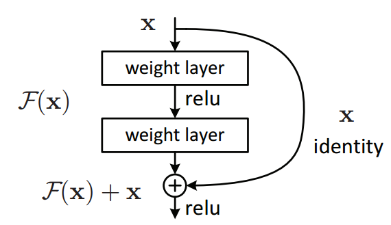
Residual Blocks, initially introduced in ResNet architectures, use **identity mappings** to mitigate gradient vanishing:
- **Shortcut Connection**: A direct identity mapping (short skip or "shortcut" connection) bypasses one or more convolutional layers, allowing the network to learn residual features $F(x) - x$.
- **Addition Operation**: The output of the shortcut connection is element-wise added to the output of the convolutional layers, creating the residual mapping, which is then passed through an activation function.
#### Code Example: Residual Block
Here is the Python code:
```python
import tensorflow as tf
def residual_block(x, filters, kernel_size=(3, 3), strides=(1, 1)):
# Shortcut connection
shortcut = x
# Main path
x = tf.keras.layers.Conv2D(filters, kernel_size, strides=strides, padding='same')(x)
x = tf.keras.layers.BatchNormalization()(x)
x = tf.keras.layers.Activation('relu')(x)
x = tf.keras.layers.Conv2D(filters, kernel_size, padding='same')(x)
x = tf.keras.layers.BatchNormalization()(x)
# Adding shortcut to main path
x = tf.keras.layers.add([shortcut, x])
x = tf.keras.layers.Activation('relu')(x) # Applying the activation after the addition
return x
```
### Skip Connections
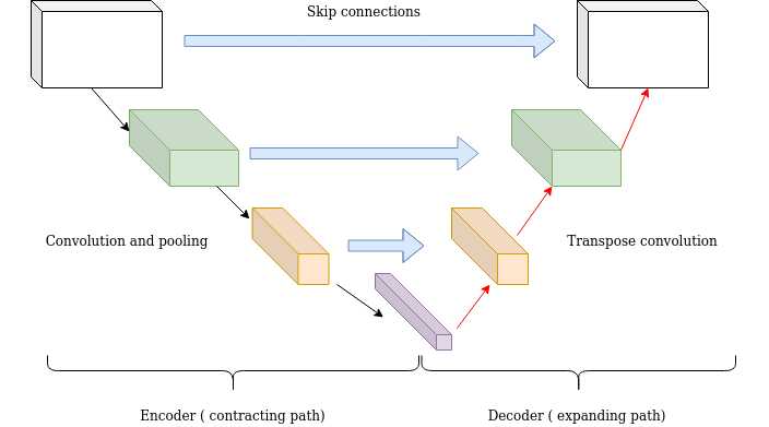
- **Complete Feature Maps**: Rather than individual channels or units, skip connections in dense (fully-connected) and convolutional layers link entire feature maps.
- **Summation or Concatenation**: While summation is common, concatenation allows for additional nonlinearities to capture more expressive power.
**Practical Applications:**
- **U-Net Architectures**: Adapted for tasks such as biomedical image segmentation.
- **DenseNets**: Every layer is connected to every other layer in a feed-forward fashion.
- **ResNeXt**: Combines the ResNet and Inception paradigms with multi-branch architectures, streamlining and enhancing information flow.
### Code Example: Skip Connection
Here is the Python code:
```python
import tensorflow as tf
# Assume x and y are tensors of compatible shapes for direct sum or concatenation
# Option 1: Summation
z1 = x + y
# Option 2: Concatenation (along channel axis)
z2 = tf.keras.layers.Concatenate()([x, y])
# Proceed with activation
z1 = tf.keras.layers.Activation('relu')(z1)
z2 = tf.keras.layers.Activation('relu')(z2)
```
#### Explore all 95 answers here 👉 [Devinterview.io - Neural Networks](https://devinterview.io/questions/machine-learning-and-data-science/neural-networks-interview-questions)