https://github.com/egonmedhatten/beta-kde
Beta Kernel Density Estimation compatible with Scikit-learn
https://github.com/egonmedhatten/beta-kde
beta-kernel boundary-bias kde kernel-density-estimation
Last synced: 6 months ago
JSON representation
Beta Kernel Density Estimation compatible with Scikit-learn
- Host: GitHub
- URL: https://github.com/egonmedhatten/beta-kde
- Owner: egonmedhatten
- License: bsd-3-clause
- Created: 2025-11-19T15:23:02.000Z (8 months ago)
- Default Branch: main
- Last Pushed: 2025-12-03T20:45:50.000Z (7 months ago)
- Last Synced: 2025-12-27T10:47:06.858Z (7 months ago)
- Topics: beta-kernel, boundary-bias, kde, kernel-density-estimation
- Language: Python
- Homepage: https://egonmedhatten.github.io/beta-kde/
- Size: 4.07 MB
- Stars: 0
- Watchers: 0
- Forks: 0
- Open Issues: 0
-
Metadata Files:
- Readme: README.md
Awesome Lists containing this project
README
# beta-kde: Boundary-Corrected Kernel Density Estimation
[](https://badge.fury.io/py/beta-kde)
[](https://opensource.org/licenses/BSD-3-Clause)
[](https://github.com/egonmedhatten/beta-kde/actions)
[](https://mybinder.org/v2/gh/egonmedhatten/beta-kde/HEAD?urlpath=%2Fdoc%2Ftree%2Fexamples%2Ftutorial.ipynb)
**Fast, finite-sample boundary correction for data strictly bounded in [0, 1].**
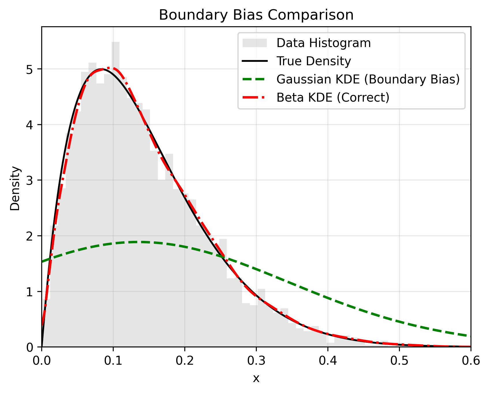
`beta-kde` is a Scikit-learn compatible library for Kernel Density Estimation (KDE) using the Beta kernel approach (Chen, 1999). It fixes the **Boundary Bias** problem inherent in standard Gaussian KDEs, where probability mass "leaks" past the edges of the data (e.g., below 0 or above 1).
## 📊 The Problem vs. The Solution
Standard KDEs smooth data blindly, ignoring bounds. `beta-kde` uses asymmetric Beta kernels that naturally adapt their shape near boundaries to prevent leakage.
## 🚀 Key Features
* **Boundary Correction:** Zero leakage. Probability mass stays strictly within the defined bounds.
* **Fast Bandwidth Selection:** Implements the **Beta Reference Rule**, a closed-form $\mathcal{O}(1)$ selector.
It matches the accuracy of expensive Cross-Validation but is **orders of magnitude faster**.
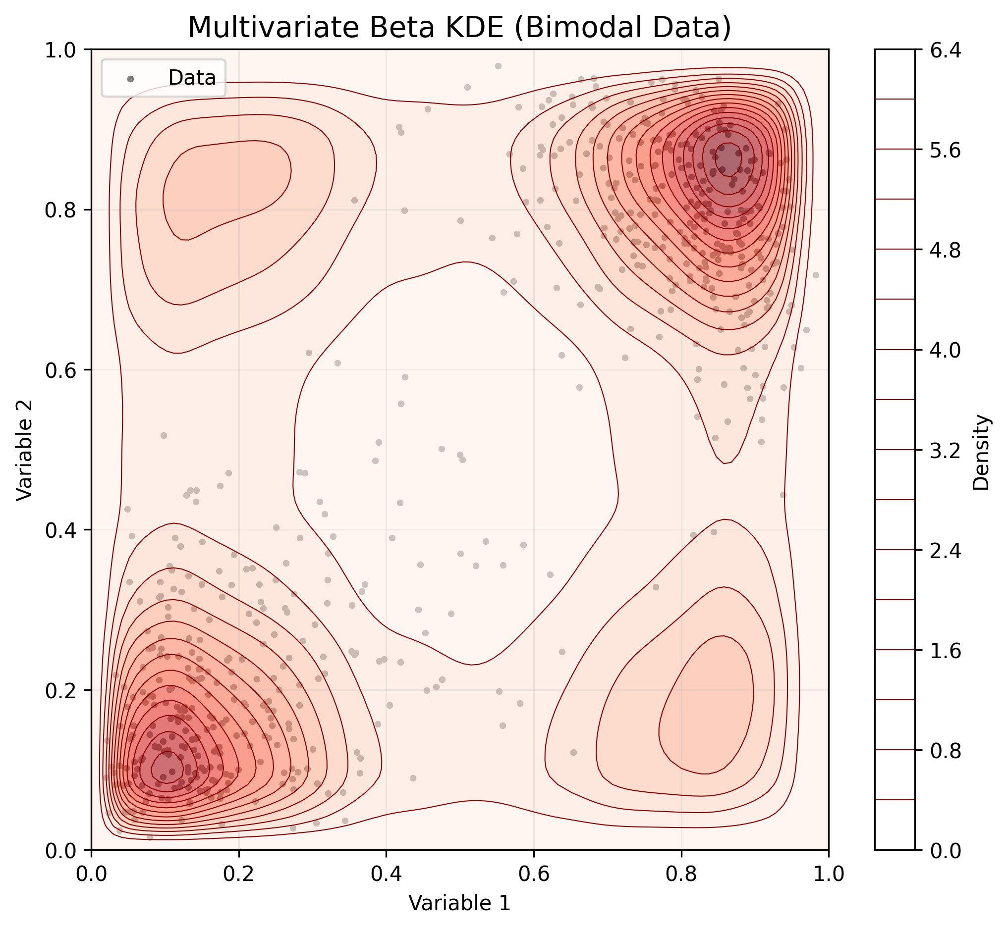
* **Multivariate Support:** Models multivariate bounded data using a **Non-Parametric Beta Copula**.
* **Scikit-learn API:** Drop-in replacement for `KernelDensity`. Fully compatible with `GridSearchCV`, `Pipeline`, and `cross_val_score`.
## 📦 Installation
```bash
pip install beta-kde
```
## ⚡ Quick Start
💡 **See the [Tutorial Notebook](https://github.com/egonmedhatten/beta-kde/blob/main/examples/tutorial.ipynb) for detailed examples, including visualization and classification.**
1. Univariate Data (The Standard Case)
BetaKDE enforces Scikit-learn's 2D input standard (n_samples, n_features).
```python
import numpy as np
from beta_kde import BetaKDE
import matplotlib.pyplot as plt
# 1. Generate bounded data (e.g., ratios or probabilities)
np.random.seed(42)
X = np.random.beta(2, 5, size=(100, 1)) # Must be 2D column vector
# 2. Fit the estimator
# 'beta-reference' is the fast, default rule-of-thumb from the paper
kde = BetaKDE(bandwidth='beta-reference', bounds=(0, 1))
kde.fit(X)
print(f"Selected Bandwidth: {kde.bandwidth_:.4f}")
# 3. Score samples
# Use normalized=True to get exact log-likelihoods (integrates to 1.0).
# Default is False for speed (returns raw kernel density values).
log_density = kde.score_samples(np.array([[0.1], [0.5], [0.9]]), normalized=True)
# 4. Plotting convenience
fig, ax = kde.plot()
plt.show()
```
2. Multivariate Data (Copula)
For multidimensional data, BetaKDE fits marginals independently and models dependence using a Copula.
```python
# Generate correlated 2D data
X_2d = np.random.rand(200, 2)
# Fit (automatically uses Copula for n_features > 1)
kde_multi = BetaKDE(bandwidth='beta-reference')
kde_multi.fit(X_2d)
# Returns log-likelihood of the joint distribution
scores = kde_multi.score_samples(X_2d)
# Plotting convenience (in the multi-variate case, this plots the marginal densities)
fig, ax = kde.plot()
plt.show()
```
### 3. Scikit-learn Compatibility (e.g. Hyperparameter Tuning)
`beta-kde` is a fully compliant Scikit-learn estimator. You can use it in Pipelines or with `GridSearchCV` to find the optimal bandwidth.
*Note: The estimator automatically handles normalization during scoring to ensure valid statistical comparisons.*
```python
from sklearn.model_selection import GridSearchCV
# Define a grid of bandwidths to test
param_grid = {
'bandwidth': [0.01, 0.05, 0.1, 'beta-reference']
}
# Run Grid Search
# n_jobs=-1 is recommended to parallelize the numerical integration
grid = GridSearchCV(
BetaKDE(),
param_grid,
cv=5,
n_jobs=-1
)
grid.fit(X)
print(f"Best Bandwidth: {grid.best_params_['bandwidth']}")
print(f"Best Log-Likelihood: {grid.best_score_:.4f}")
```
## ⚡ Performance & Normalization
Unlike Gaussian KDEs, Beta KDEs do not integrate to 1.0 analytically. Normalization requires numerical integration, which can be computationally expensive. beta-kde handles this smartly:
* **Lazy Loading:** fit(X) is fast and does not compute the normalization constant.
* **On-Demand:** The integral is computed and cached only when you strictly need it (e.g., calling kde.score(X) or kde.pdf(X, normalized=True)).
* **Flexible Scoring:**
* score_samples(X, normalized=False) (Default): Fast. Best for clustering, relative density comparisons, or plotting shape.
* score(X): Accurate. Always returns the normalized total log-likelihood. Safe for use in GridSearchCV.
## 🆚 Why use beta-kde?
If your data represents percentages, probabilities, or physical constraints (e.g., $x \in [0, 1]$), standard KDEs are mathematically incorrect at the edges.
| Feature | `sklearn.neighbors.KernelDensity` | `beta-kde` |
| :--- | :--- | :--- |
| **Kernel** | Gaussian (Symmetric) | Beta (Asymmetric) |
| **Boundary Handling** | **Biased** (Leaks mass < 0) | **Correct** (Strictly $\ge 0$) |
| **Bandwidth Selection** | Gaussian Reference Rule | **Beta Reference Rule** |
| **Multivariate** | Symmetric Gaussian Blob | Flexible Non-Parametric Copula |
| **Speed (Prediction)** | Fast (Tree-based) | Moderate (Exact summation) |
### ⚠️ Important Usage Notes
1. **Strict Input Shapes:** Input X must be 2D. Use X.reshape(-1, 1) for 1D arrays. This constraint prevents accidental application of univariate estimators to multivariate data.
2. **Computational Complexity:** This is an exact kernel method.
* Raw density (normalized=False) is fast.
* Exact probabilities (normalized=True) require a one-time integration cost per fitted model.
* Recommended for datasets with $N < 50,000$.
3. **Bounds:** You must specify bounds if your data is not in $[0, 1]$. The estimator handles scaling internally.
### 📚 References
1. Chen, S. X. (1999). Beta kernel estimators for density functions. Computational Statistics & Data Analysis, 31(2), 131-145.
### License
BSD 3-Clause License