https://github.com/felixfaisal/ml-notes
This Repository will contain notes of my current machine learning course
https://github.com/felixfaisal/ml-notes
Last synced: 26 days ago
JSON representation
This Repository will contain notes of my current machine learning course
- Host: GitHub
- URL: https://github.com/felixfaisal/ml-notes
- Owner: felixfaisal
- Created: 2021-05-25T11:08:24.000Z (over 4 years ago)
- Default Branch: main
- Last Pushed: 2021-05-25T12:33:49.000Z (over 4 years ago)
- Last Synced: 2025-02-05T17:11:40.079Z (12 months ago)
- Size: 23.4 KB
- Stars: 0
- Watchers: 2
- Forks: 0
- Open Issues: 0
-
Metadata Files:
- Readme: README.md
Awesome Lists containing this project
README
# Supervised Learning
- In supervised learning, the labelled training data provide the basis for learning.
- The process of learning from the training data by a machine can be related to an expert supervising the learning process of a student.
- Here the expert is the training data.
- Training data is the past information with known value of class field or ‘label’.
- Unsupervised learning uses no labelled data.
- Semi-supervised learning uses a small amount of labelled data.
## Supervised vs Unsupervised Learning

## Classification Model
- When we try to predict a categorical or nominal variable, the problem is known as a classification problem.
- Here, the problem centres around assigning a label or category or class to the test data on the basis of the label or category or class information imparted by training data.
- Classification is a type of supervised learning where a target feature, i.e. A categorical type, is predicted for test data on the basis of information obtained from training data.
- This categorical feature is known as class.
## Classification with learning steps

## Common Classification Algorithms
1. **k-Nearest Neighbour (kNN)**
2. **Decision tree**
3. **Random forest**
4. **Support Vector Machine (SVM)**
5. **Naive Bayes classifier**
## Origins of KNN
- Nearest Neighbors have been used in statistical estimation and pattern recognition already in the beginning of 1970’s (non- parametric techniques).
- The method prevailed in several disciplines and still it is one
of the top 10 Data Mining algorithm.
- It’s how people judge by observing our peers.
- We tend to move with people of similar attributes so does data.
### Definition
- **K-Nearest Neighbor** is considered a lazy learning algorithm that classifies data sets based on their similarity with neighbors.
- “K” stands for number of data set items that are considered for the classification.
- Ex: Image shows classification for
different k-values.

- For the given attributes `A={X1, X2….. XD}` Where **D** is the dimension of the data, we need to predict the corresponding classification group `G={Y1,Y2…Yn}` using the proximity metric over **K** items in **D** dimension that defines the closeness of association such that `X € RD` and `Yp € G`.
### That is

- Attribute A={Color, Outline, Dot}
- Classification Group, G={triangle, square}
- D=3, we are free to choose K value.
## Proximity Metric
- Definition: Also termed as “Similarity Measure” quantifies the association among different items.
- Following is a table of measures for different data items:

## Voronoi Diagram
- A Voronoi diagram is a partitioning of a plane into regions based on distance to points in a specific subset of the plane.
- Here, k=1.

## KNN Example

### Proximity Metric
For the numeric data let us consider some distance measures
- Manhattan Distance

Ex: Given X = {1,2} & Y = {2,5}
Manhattan Distance = dist(X,Y) = |1-2|+|2-5|
= 1+3
= 4
- Euclidean Distance

## KNN in Action
- Consider the following data: A={weight,color} G={Apple(A), Banana(B)}
- We need to predict the type of a
fruit with: weight = 378 color = red

- Assign color codes to convert into numerical data

- Let’s label Apple as “A” and Banana as “B”
- Using K=3,
Our result will be,

## KNN Properties
- K-NN is a lazy algorithm
- The processing defers with respect to K value.
- Result is generated after analysis of stored data.
- It neglects any intermediate values.
### Advantages
- Can be applied to the data from any distribution,
for example, data does not have to be separable with a linear boundary
- Very simple and intuitive
- Good classification if the number of samples is large enough
### Disadvantages
- Dependent on K Value
- stage is computationally expensive
- Need large number of samples for accuracy
## DECISION TREE
- This is one of the most adopted algorithms for classification.
- It builds a model in the form of a tree structure.
- A decision tree is used for multi-dimensional analysis with multiple classes and is characterized by ease of interpretation of rules and fast execution.
- The goal of decision tree learning is to create a model that predicts the value of the output variable based on the input variables in the feature vector.
- It contains a decision node and a leaf node.
- Each decision node corresponds to one of the feature vector.
- From every node, there are edges to children, wherein there is an edge for each of the possible values of the feature associated with the node.
- The output variable is determined by following a path that starts at the root and is guided by the values of the input variables.
- Decision trees can be used for both classification and regression.
## Decision Tree to Play Tennis

## Example: Will a Person Buy a computer?

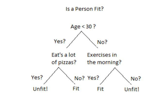
## Example: Is a Person Fit?
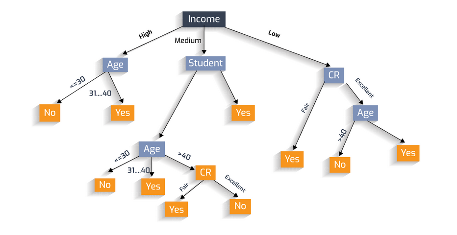
## Example Should loan be sactioned
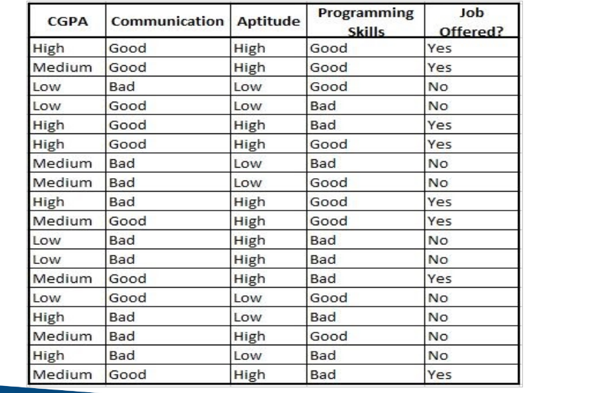
## Training Data for GTS Recruitment
## Entropy of a decision tree
- Entropy, as it relates to machine learning, is a measure of the randomness in the information being processed.
- The higher the entropy, the harder it is to draw any conclusions from that information.

- Ex: For class ‘Job Offered?’ we have two values: Yes and No.
- Pi values for Yes= 8/18 = 0.44 & No= 10/18= 0.56
Entropy(S) = -0.44 log2(0.44) – 0.56 log2(0.56)
= 0.99
## Information Gain on a Decision Tree
- The information gain is created on the basis of the decrease in entropy(S) after a data set is split according to a particular attribute(A).
- Constructing a decision tree is all about finding an attribute that returns the highest information gain.
- If information gain is 0, it means that there is no reduction in entropy due to split of the data set according to that particular feature.
- The maximum amount of information gain which may happen is the entropy of the data set before the split.
- Information gain for a particular feature A is calculated by the difference in entropy before a split(Sbs) with the entropy after the split(Sas).
- Information gain(S, A) = Entropy(Sbs) – Entropy(Sas)
- For weighted summation, the proportion of examples falling into each partition is used as weight.
- Entropy(Sas) = ∑ (i=1 to n) wi Entropy(pi)
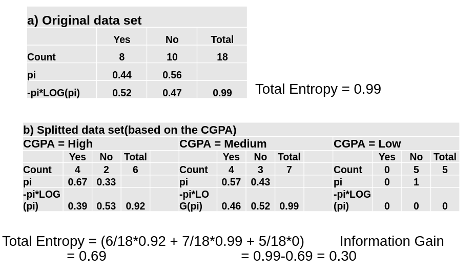
c) Splitted data set(based on ‘Communication’)
Communication = ‘Good’ Communication = ‘Bad’
Total Entropy = 0.63 Information Gain = 0.36
d) Splitted data set(based on ‘Aptitude’)
Aptitude = ‘High’ Aptitude = ‘Low’
Total Entropy = 0.52 Information Gain = 0.47(Entropy=0)
e) Splitted data set(based on ‘Programming Skills’)
Programming Skills = ‘Good’ Programming Skills = ‘Bad’
Total Entropy = 0.95 Information Gain = 0.04
## Avoid Overfitting in Decision Tree Pruning
- The decision tree algorithm, unless a stopping criterion is applied, may keep growing indefinitely.
- To prevent a decision tree getting overfitted to the training data, pruning of the decision tree is essential.
- Pruning a decision tree reduces the size of the tree such that the model is more generalized and can classify unknown and unlabeled data in a better way.
- Pre-pruning: Stop growing the tree before it reaches perfection.
- Post-pruning: Allow the tree to grow entirely and then post-prune some of the branches from it.
## Random Forest Model
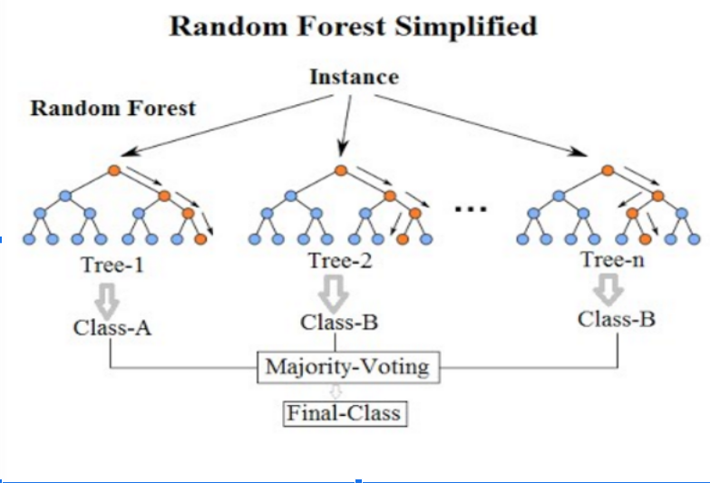
- It is an ensemble classifier, i.e., a combining classifier that uses and combines many decision tree classifiers.
- Ensembling is usually done using the concept of bagging with different feature sets.
- The reason for using large number of trees in random forest is to train the trees enough such that contribution from each feature comes in a number of models.
- After the random forest is generated by combining the trees, majority vote is applied to combine the output of the different trees.
- Ensembled model yields better result than decision trees.
## Random Forst Algorithm
The algorithm works as follows:
1. If there are N variables or features in the input data set, select a subset of ‘m’ (m