https://github.com/finsberg/fenicsx-beat
https://github.com/finsberg/fenicsx-beat
cardiac ecg electrophysiology fenicsx finite-element-analysis monodomain-model
Last synced: 10 months ago
JSON representation
- Host: GitHub
- URL: https://github.com/finsberg/fenicsx-beat
- Owner: finsberg
- License: mit
- Created: 2024-04-09T08:12:48.000Z (over 2 years ago)
- Default Branch: main
- Last Pushed: 2024-12-18T18:12:06.000Z (over 1 year ago)
- Last Synced: 2024-12-18T19:26:00.331Z (over 1 year ago)
- Topics: cardiac, ecg, electrophysiology, fenicsx, finite-element-analysis, monodomain-model
- Language: Python
- Homepage: https://finsberg.github.io/fenicsx-beat/
- Size: 9.2 MB
- Stars: 1
- Watchers: 1
- Forks: 0
- Open Issues: 2
-
Metadata Files:
- Readme: README.md
- Contributing: CONTRIBUTING.md
- License: LICENSE
Awesome Lists containing this project
README

# fenicsx-beat
Cardiac electrophysiology research uses computational modeling to study heart rhythm disorders and test therapies.
This tool, fenicsx-beat, is a cardiac electrophysiology simulator built specifically for the FEniCSx platform. It provides a dedicated and easy-to-use tool for researchers already using [FEniCSx](https://fenicsproject.org) to perform simulations based on the Monodomain model.
- Source code: https://github.com/finsberg/fenicsx-beat
- Documentation: https://finsberg.github.io/fenicsx-beat
## Install
You can install the library with `pip`
```
python3 -m pip install fenicsx-beat
```
or with `conda`
```
conda install -c conda-forge fenicsx-beat
```
Note that installing with `pip` requires [FEniCSx already installed](https://fenicsproject.org/download/)
Also that to run most of the examples you will need to install additional dependencies which can be done using the command
```
python3 -m pip install fenicsx-beat[demos]
```
## Getting started
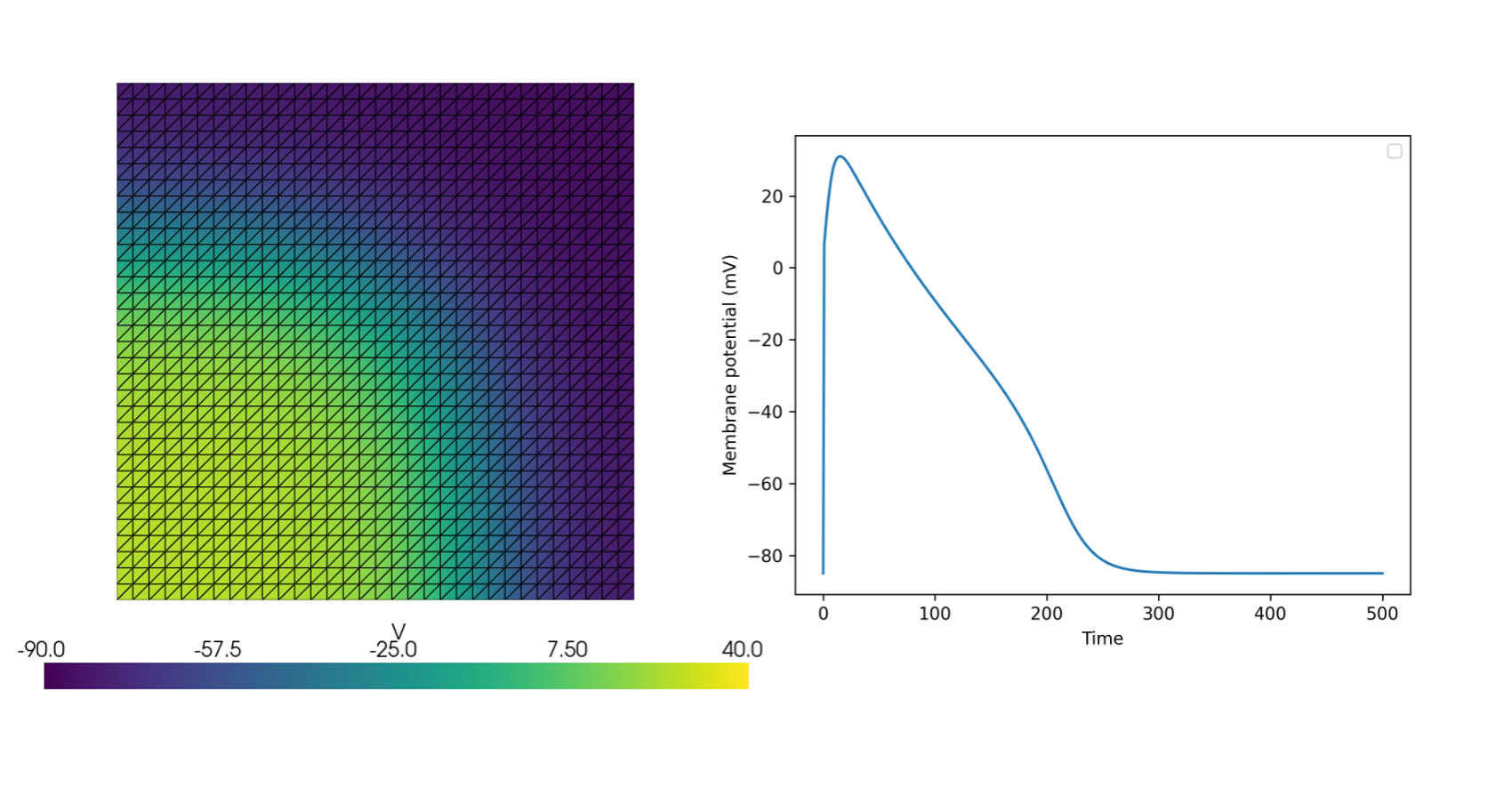
The following minimal example demonstrates simulating the Monodomain model on a unit square domain using a modified FitzHugh-Nagumo model
```python
import shutil
import matplotlib.pyplot as plt
import numpy as np
from mpi4py import MPI
import dolfinx
import ufl
import beat
# MPI communicator
comm = MPI.COMM_WORLD
# Create mesh
mesh = dolfinx.mesh.create_unit_square(comm, 32, 32, dolfinx.cpp.mesh.CellType.triangle)
# Create a variable for time
time = dolfinx.fem.Constant(mesh, dolfinx.default_scalar_type(0.0))
# Define forward euler scheme for solving the ODEs
# This just needs to be a function that takes the current time, states, parameters and dt
# and returns the new states
def fitzhughnagumo_forward_euler(t, states, parameters, dt):
s, v = states
(
c_1,
c_2,
c_3,
a,
b,
v_amp,
v_rest,
v_peak,
stim_amplitude,
stim_duration,
stim_start,
) = parameters
i_app = np.where(
np.logical_and(t > stim_start, t < stim_start + stim_duration),
stim_amplitude,
0,
)
values = np.zeros_like(states)
ds_dt = b * (-c_3 * s + (v - v_rest))
values[0] = ds_dt * dt + s
v_th = v_amp * a + v_rest
I = -s * (c_2 / v_amp) * (v - v_rest) + (
((c_1 / v_amp**2) * (v - v_rest)) * (v - v_th)
) * (-v + v_peak)
dV_dt = I + i_app
values[1] = v + dV_dt * dt
return values
# Define space for the ODEs
ode_space = dolfinx.fem.functionspace(mesh, ("P", 1))
# Define parameters for the ODEs
a = 0.13
b = 0.013
c1 = 0.26
c2 = 0.1
c3 = 1.0
v_peak = 40.0
v_rest = -85.0
stim_amplitude = 100.0
stim_duration = 1
stim_start = 0.0
# Collect the parameter in a numpy array
parameters = np.array(
[
c1,
c2,
c3,
a,
b,
v_peak - v_rest,
v_rest,
v_peak,
stim_amplitude,
stim_duration,
stim_start,
],
dtype=np.float64,
)
# Define the initial states
init_states = np.array([0.0, -85], dtype=np.float64)
# Specify the index of state for the membrane potential
# which will also inform the PDE solver later
v_index = 1
# We can also check the solution of the ODE
# by solving the ODE for a single cell
times = np.arange(0.0, 1000.0, 0.1)
values = np.zeros((len(times), 2))
values[0, :] = np.array([0.0, -85.0])
for i, t in enumerate(times[1:]):
values[i + 1, :] = fitzhughnagumo_forward_euler(t, values[i, :], parameters, dt=0.1)
fig, ax = plt.subplots()
ax.plot(times, values[:, v_index])
ax.set_xlabel("Time")
ax.set_ylabel("States")
ax.legend()
fig.savefig("ode_solution.png")
# Now we set external stimulus to zero for ODE
parameters[-3] = 0.0
# and create stimulus for PDE
stim_expr = ufl.conditional(ufl.And(ufl.ge(time, 0.0), ufl.le(time, 0.5)), 600.0, 0.0)
stim_marker = 1
cells = dolfinx.mesh.locate_entities(
mesh, mesh.topology.dim, lambda x: np.logical_and(x[0] <= 0.5, x[1] <= 0.5)
)
stim_tags = dolfinx.mesh.meshtags(
mesh,
mesh.topology.dim,
cells,
np.full(len(cells), stim_marker, dtype=np.int32),
)
dx = ufl.Measure("dx", domain=mesh, subdomain_data=stim_tags)
I_s = beat.Stimulus(expr=stim_expr, dZ=dx, marker=stim_marker)
# Create PDE model
pde = beat.MonodomainModel(time=time, mesh=mesh, M=0.001, I_s=I_s, dx=dx)
# Next we create the PDE solver where we make sure to
# pass the variable for the membrane potential from the PDE
ode = beat.odesolver.DolfinODESolver(
v_ode=dolfinx.fem.Function(ode_space),
v_pde=pde.state,
fun=fitzhughnagumo_forward_euler,
init_states=init_states,
parameters=parameters,
num_states=len(init_states),
v_index=1,
)
# Combine PDE and ODE solver
solver = beat.MonodomainSplittingSolver(pde=pde, ode=ode)
# Now we setup file for saving results
# First remove any existing files
shutil.rmtree("voltage.bp", ignore_errors=True)
vtx = dolfinx.io.VTXWriter(mesh.comm, "voltage.bp", [pde.state], engine="BP5")
vtx.write(0.0)
# Finally we run the simulation for 400 ms using a time step of 0.01 ms
T = 400.0
t = 0.0
dt = 0.01
i = 0
while t < T:
v = solver.pde.state.x.array
solver.step((t, t + dt))
t += dt
if i % 500 == 0:
vtx.write(t)
i += 1
vtx.close()
```
See more examples in the [documentation](https://finsberg.github.io/fenicsx-beat)
## License
MIT
## Need help or having issues
Please submit an [issue](https://github.com/finsberg/fenicsx-beat/issues)