https://github.com/gabboraron/computer_aided_solution_processing
In the lecture course, students learn elements of supervised machine learning and mathematical optimization with emphasis on regression methods and combinatorial optimization. The course also discusses methods for estimation of machine learning model's predictive performance, feature selection, optimization of model's structure, as well as practical applications of the methods.
https://github.com/gabboraron/computer_aided_solution_processing
deep-learning machine-learning regression-models riga-technical-university
Last synced: 6 months ago
JSON representation
In the lecture course, students learn elements of supervised machine learning and mathematical optimization with emphasis on regression methods and combinatorial optimization. The course also discusses methods for estimation of machine learning model's predictive performance, feature selection, optimization of model's structure, as well as practical applications of the methods.
- Host: GitHub
- URL: https://github.com/gabboraron/computer_aided_solution_processing
- Owner: gabboraron
- License: mpl-2.0
- Created: 2022-02-07T08:12:51.000Z (almost 4 years ago)
- Default Branch: main
- Last Pushed: 2022-04-25T10:29:32.000Z (over 3 years ago)
- Last Synced: 2025-04-06T15:36:53.331Z (9 months ago)
- Topics: deep-learning, machine-learning, regression-models, riga-technical-university
- Homepage: https://vitalflux.com/
- Size: 92.8 KB
- Stars: 0
- Watchers: 2
- Forks: 1
- Open Issues: 0
-
Metadata Files:
- Readme: README.md
- License: LICENSE
Awesome Lists containing this project
README
# Computer Aided Solution Processing
- [list of courses about deep learning](https://github.com/josephmisiti/awesome-machine-learning/blob/master/courses.md)
- [Andrew Ng YouTube Lecture Collection | Machine Learning - Stanford](https://www.youtube.com/playlist?list=PLA89DCFA6ADACE599)
- [Stanford CS229: Machine Learning | Autumn 2018](https://www.youtube.com/playlist?list=PLoROMvodv4rMiGQp3WXShtMGgzqpfVfbU)
- [free books about deep learning](https://github.com/josephmisiti/awesome-machine-learning/blob/master/books.md)
**Requirements:**
- test after each lecture 10-15 min
- micro projects
-----
## Topic 1 - Introduction
## Topic 2 - Notation/ Linear Regression / Least Squares Method
### regression types
In supervised learning, if the output `y` is real-valued quantitative, the problem is called regression.
> **Notation**
> - `n` - number of datapoints, the exxamples in training dataset
> - `m` - imput variables
> - `j` - index of columns
> - `i` - index of rows
> - `x``j` - `j`-th input variable
> - `x``i` - `i`-th row vector
> - `y` output variable
### Regression problem
```
____________________
x -> | system under study | -> y
_____________________
```
When we are studying a behavior of some system, we observe `m` different input variables (features) `x = (x1, x2, ..., xm)` and a quantitative output variable `y`.
`y = h(x) + ε`
`h` represents systematic information that `x` provides about `y`. `ε` is just noise that doesn’t give us any useful information.
- the utput `y` contain noise too!
- we do not know function `h(x)`
We create our function about `x` which gives us a prediction about `y` this will be: `ŷ = f(x)` and can simulate `h`.
### Linear regression
**Linear regression assumes that the relationship between `x` and `y` is liner (simply a sum of the features): `y = a0 + a1x1 + a2x2 + ... + amxm + ε` or **
Now we just have to find the values of this sum, and this is much easier than find the original function. For linear models, we need to estimate the parameters `a0, a1, ..., am` such that it predicts `y` with the least error.
#### Simplest case
one feature => `m=1` => this means just a line:
`ŷ = a0 + a1x`
- `a0` - determines `y` value when `x = 0`; *ex: when the line crosses the `y` axis - y-intercept*
- `a1` determines the slope of the line
We need to train the model – we need a procedure, that uses the training data to estimate model’s parameters `a0`, `a1` => ***The line should be in minimal distance from all the data points at the same time***
**Criterions:**
- minimize absolute residuals
- minimize residuals with sum of squeres
**How to do it:**
1. try to guess - not so useful
2. [search iteratively](https://towardsdatascience.com/linear-regression-using-gradient-descent-97a6c8700931) - so much time...
3. [least squeres method](https://setosa.io/ev/ordinary-least-squares-regression/)
model: `ŷ = a0 + a1x` - from `x`calculate `y`, sust as simple with the criteria: ^2\right)) and `li = yi – ŷi`
if we replace `ŷ` and `li` then we got: ^2\right))
To find the minimal of the function we need to derivate it, on `a0` and `a1` too!
- })
- })
***in practice the differentiation step is skipped, i.e., we can go directly to the system of equations***
we got a linear system of equations:
- 
- 
training dataset: `x` is `Exam`
```
Quiz Exam
5.6 5.0
6.5 7.1
6.8 8.4
6.9 7.3
7.0 7.8
7.4 8.1
8.0 7.4
8.3 8.9
8.7 9.0
9.0 10.0
```
put the traing numbers into the equations... OR use Gaussian elimination
The given line will be the best with this criteria! If we change it then this not will be true!
## Topic 3 - Linear regression | Least square method | simple model evaluation
### linear regressions
- `ŷ = a0+a1 x`
- `ŷ = a0 + a1x + a2x^2`
- `ŷ = a0 + a1x + ... + a2x^d`
#### quadratic polynomial (d = 2 )
- equation for parabola: `ŷ = a0 + a1x + a2x2`
- when a2 -> 0 shape of parabola approaches straight line
now if we have a dataset with `x` and `y`; at least with 14 rows (`n=14`); we want to calculate `a0`, `a1` and `a2` from `ŷ = a0 + a1x + a2x^2`. As previously before, now we have to use `li` in criteria `S` and `ŷ` model in criteria. With this we got: !S\ =\ \sum_{i=1}^{n}{(y_i-a_0{-a}_1x_i-a_2x_i^2)}^2]https://latex.codecogs.com/gif.latex?S\%20=\%20\sum_{i=1}^{n}{(y_i-a_0{-a}_1x_i-a_2x_i^2)}^2) we have to minimize with the Residual Sum of Squares method.
Now we can take partial derivatives of `a0`, `a1`, `a2`
- )
- })
- })
take eqal with 0, and let's make a linear system of equations from it.
- 
- 
- 
Now we got `a0`, `a1`, `a2`. If we get an `x` value, we can calculate the `ŷ`.
Any features can be written as a sum of features.
***But what if we need something more complex than just a sum of features?***
#### Least Squares Method generalized
#### how good is our model?
> ***always smaller values are better***
Usually get values on `[0,1]` but if the test dataset is different then training data then might be `-1`, so, in that case, don't use that model **!**
more about different models: https://methods.sagepub.com/images/virtual/heteroskedasticity-in-regression/p53-1.jpg
[Mean Squared Error VS R-Squared](https://vitalflux.com/mean-square-error-r-squared-which-one-to-use/)
## Topic 4 - Model evaluation and selection - Resampling methods
> - how good is a model for oour dataset
> - how to choose the best model for the dataset?

- straight line: the model is too simple - R^2: 0.6
- when the courve fit exactly on data points: overfitting: R^2: 0.99
*When the number of parameters is equal to the number of data points the curve goes exactly through all the points*
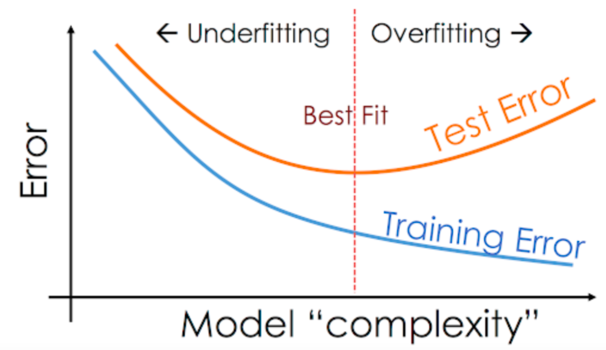
prediction error is nknown, just training error can be calculated, but we can estimate prediction error!
error means: SAE, MAE, SSE, MSE, RMSE
**Advantages of simple models:**
- Better predictive performance (except if underfitted)
- A simple model might use fewer features => fewer measurements or other kinds of data gathering
- faster
- needs less computer memory
- Simpler models are easier to visualize and interpret
> **Idea**
>
> *We know that when we use a model for prediction, we calculate y for given x which may not be (and usually is not) given in the training dataset. What if we could “simulate” this process? We could use additional evaluation dataset which is not included in the training dataset.*
### Validation set and test set
- dataset is used for model selection the dataset is called validation set
- it is used for final estimation of prediction error it is called test set
**The aims of model selection and final evaluation:**
- **Model selection:** select the best model by evaluating predictive performance of modelscandidates - relative differences between evaluations of different models
- **Final estimation of the true prediction error:** the true prediction error as closely as possible in this way giving information about the expected error of the model
both cases we can use resampling methods: ***evaluate the model on additional data that was not included in the training*** these additional data points would not be included in the training set, not even in model building
this can happen by:
- Additionally generated
- Simply subtracted from the already existing full dataset
#### The three datasets method
- divide the whole dataset into three subsets (or two, if either validation or testing is not required)
- the division is usually 60:20:20 or 70:30
#### Hold-Out method
- Each model-candidate is evaluated using the validation set
- at given `x` we calculate the error between model’s predicted `ŷ` value and the `y` value given in the validation dataset
- ***In the end, the one “best” model is evaluated in the same as using the test set***
- the order of the data points is randomized!
- **Advantages:**
- Easy to implement and use
- **Efficiency of computations** – nothing is to be computed more than once
- **Disadvantages:**
- **can't use on small datasets!**
- Considerably reduces the size of the training data
- We can get “unlucky” data point combinations in any of the set

#### Cross-Validation
##### k-fold Cross-Validation
- All examples of the full dataset are randomly reordered
- divided in `k` subsets of equal size
- `k` iteration:
- each iteration `j`th subset is used as a test set
- other `k – 1` subset is used as a training set
- , the model is created `k` times; error is calculated `k` times => final evaluation of the model: calculating the average of the errors

##### Leave-One-Out Cross-Validation *(k = n)*
- number of iterations is equal to the number of examples
- test set always includes only one example but overall through all iterations the evaluation is done on all examples
This is a good alternative for very small datasets because you remove only one example from the training set and you evaluate the model as many times as the possible
Advantages:
- All the data is used for calculations of model parameters
- on small dataset better than Hold-out
disadvantages:
- requires k times more iterations than othe ones, so this is slow!
## Topic 5 - Alternative to the resampling methods General scheme of the whole process
## Topic 6 - Nearest Neighbors Method
### Nearest Neighbors
Using Euclidean distance method to find the distance of two different points: 2) on )
-  is the query point (a vector) - from here we calculate distances to all training examples
-  the `i`th training example - this is for which we calculate the distance
- `j` is the feature
- `m` is the total number of features
- `n` number of training datapoints
calculate the prediction `ŷ` by simple averaging of `y` over the vound `k` nearest examples: 
***Larger `k` values reduce influence of noise but smoothes-out predictions!***
To improve predictive performance of k-NN, it is recommended to normalize (rescale values to range [0,1])  or standardize each feature  where the `s` standardization is ^2%20})
> **A potential problem**: all of the `k` neighbors are taken into account with the same weight, i.e., they all have the same influence on the result. *only for `k > 1`; if `k = 1` that's the most complex method*
### Weighted nearest neighbors method
}{\sum_{i=1}^{k}w_i})
- Without weighting (uniform): 
- Inverted distance: 
- Predictive performance of `k-NN` can be considerably reduced by having too many features: - Feature subset selection might help
#### advantages
- fast learning - all the examples in memory
- very felxible - able to capture complex patterns using very simple principles
- fast update - more exaplest to training data there is no need in training a new model
#### disadvantages
- serious predictive performance issues for highly dimensional data, especially if the number of data points is small <- feature selection
- needs realatively large computational resources - the learning is fast but the prediction is slow
## Subset selection, model building, state space, heuristic search
> literature: [Trevor Hastie, Robert Tibshirani, Jerome Friedman - The Elements of Statistical Learning: Data Mining, Inference, and Prediction](https://hastie.su.domains/ElemStatLearn/)
>
> *Report & projects*
> - deadline: may 2
> - choose between report and project
> - writing a report: find a literature, write a report about the topic
> - choose 3 topics - from these one you will give one
> -
Finding a good model, by balancing between underfitting and overfitting, is not only about:
- best value for some hyperparameter
- selecting best degree for the polynomial in linear regression
- selecting best k value for k-NN method
- etc
Not all features might be useful
- Irrelevant features don’t give any useful information for prediction purposes *ex: car color when you want to estimate fuel consumption of the car*
- Redundant features strongly correlate with each other and so it might be that only one of them is actually useful *ex volume of engine (engine displacement) in cubic centimeters vs. cubic inches, or for example product’s price vs. VAT of the price*
*example: model of house price*
- *redundant: area, nr of rooms*
- *irrelevant: color of building*
- *not sure we need: floor number, nr of floors in the building*
- *we need for sure: year of construction*
In order to obtain a statistically reasonable result, the amount of data needed to support the result grows fast, it can grow even exponentially, with the dimensionality, even if you keep only the useful features, you still have too many of them
**Solutions to these problems are:**
- Remove features that are the least useful
- Use methods that transforms the data in high-dimensional space to a space of fewer dimensions, *ex: Principal Component Analysis (PCA)*
### Dimensionality reduction
> in case of linear regression, selecting the necessary features can be done either on the level of original input variables or on the level of the transformations
>
> How to find which features to use:
> - Feature subset selection because we are searching for the “best” subset of the full set of features
> - Model selection because we are choosing one “best” model from a number of possible models
> - Model building because we are building a model from the available components (features, their transformations)
>
> ***The lower is the number of examples in your dataset (compared to the number of features) the more important is the feature selection problem***
#### Feature subset selection
- “Manual” feature selection is practical only with small number of features and/or features that can be easily understood.
- While working with just a few features, the data and the model can be visualized, interpreted, and evaluated relatively easily: `nr_of_features - 1` is the dimension of the model
- to formalize this process and make it automatic:

Evaluate all possible combinations (all possible models) and choose the best. Big problem: the number of combinations of features grows exponentially.
***The number of all possible combinations is `2^m`, where `m` is the total number of features defined.*** This means a big problem if we use exhaustive search or brute force.
We need a type of search that enables us to find good combinations/models without requiring huge computational resources => Solution – use heuristics
- Advantage – significant savings of time (e.g., not days, months, or years but seconds, minutes, or hours)
- Disadvantage – such algorithms do not guarantee optimality of the results, instead they can give us good solutions in within a reasonable time. – this is usually good enough.
##### heuristic sarch
1. Initial state The combination with which we begin our search.
2. State-transition operators The available ways to modify the combination.
3. Search strategy Which combinations to evaluate and where to go next.
4. State evaluation criterion Criterion for evaluation of the created combinations.
5. Termination condition When to stop the search
typical variations:
1. Initial state - Empty set (no features included, “00000”), full set (all features included, “11111”), random subset.
2. State-transition operators - The two typical operators: addition of one feature (0 -> 1), deletion of one feature (1 -> 0). There can be also other operators, e.g., genetic algorithms use crossover and mutation
3. Search strategy -
- Hill Climbing,
- Beam Search,
- Floating Search,
- Simulated Annealing,
- imitation of evolution (in Genetic Algorithms) etc.
4. State evaluation criterion - In our case: Hold-out, Cross-Validation, MDL, AIC, AICC etc.
5. Termination condition - When none of the operators can find a better state (local minimum found). When none of the operators are applicable anymore. When a predefined number of iterations are done. When a predefined error rate is reached. When a predefined time is elapsed. Etc
#### SFS algo
1. Initial state - Empty set (no features included, “00000”).
2. State-transition operators - Addition of one feature to the model (0 -> 1)
3. Search strategy - A variation of Hill Climbing
4. State evaluation criterion - (We can use any suitable criterion)
5. Termination condition
a) When none of the operators can find a better state (local minimum found).
b) When none of the operators are applicable (i.e., for SFS this means that the state with all bits equal to 1 is reached). [In next slides, the (b) version of the algorithm is explained.]

##### Bit representation:
a linear regression modell look like this: `ŷ = a0 + a1x1 + a2x2 + a3x3 + a4x4 + a5x5` each `x` is a feature, int his case we have 5 features, so we need 5 bits: `00000` is where none of the features is used, and `11111` where all of them.
# Genetic Algorithms (GA)
- global optimization
> - search the space globally in multiple regions at the same time as well as by doing jumps of different lengths
> - local minima problem is not as pronounced
## Genetic algorithms have many variations and they are widely applicable to different optimization problems
The basic components:
1. initial state: empty set: no features: `0000` or full state: `1111`
2. state-transition operations: addtion of one feature, deletion of a feature *using crossover mutation*
3. search strategy: Hill Climbing, Beam Search, Floating Search, Simulated Annealing, imitation of evolution
4. State evaluation criterion In our case: Hold-out,
5. Termination condition When none of the operators can find a better state. When a predefined number of iterations are done. When a predefined error rate is reached.
> *Note that in the case of imitation of evolution (like it is in GA), the algorithm works with multiple solutions at the same time, instead of just improving one solution (as in the algorithms from the last lecture).*
### short about natural evolution:
- Natural selection – survival of the fittest.
- Population of individuals live and reproduce in an environment of limited resources.
- The fittest individuals survive and pass their genes to offspring. The offspring are potentially even more fit to the environment than their parents.
- Less fit individuals have lower chances of surviving and getting to produce any offspring (in the amount necessary for the harshness of the environment).
- Therefore the population through generations becomes more and more fit to the environment.
- Evolution is optimization.
### implementation and terminology:
- A population of individuals where each individual is a possible solution
- Each individual is defined by its chromosome
- chromosome consists of a number of genes
- A fitness function evaluates fitness of individuals. The whole goal of the GA is to either minimize or maximize this function
> ## The general algorithm:
> 1. Randomly generate initial generation (“primordial soup”)
> 2. Evaluate all individuals (fitness estimation)
> 3. Selection – select individuals for reproduction
> 4. Crossover – selected individuals produce offspring
> 5. Mutation – small random changes in offspring
> 6. With the new generation go to step 2
>
> continues until a predefined number of generations (iterations) is reached
# Other applications of Genetic Algorithms (and other similar algorithms)
What do we need:
- How do we encode the structure that must be optimized (so that it can be manipulated using unified and simple crossover and mutation operators)
- How do we quantitatively estimate the quality of the structure – its “nearness” to our optimization goal (development of the fitness function)
In feature subset selection they were:
- A string of bits (inclusion/exclusion of features)
- A function for estimating model’s prediction error
## Possibilities in applying Genetic Algorithms:
> ### Linear structure with fixed number of elements
> #### Optimization of combination of elements
> - Genes are bits
> - Examples – feature subset selection, mathematical transformation selection, “knapsack” problem etc.
> - + bits can be used to represent more than two values
>
> #### Optimization of element numeric values
> - Genes are real numbers or integers
> - Examples – real-valued parameter optimization of configuration for any system or construction
>
> #### Optimization of element order
> - Genes are identifiers
> - Examples – pathfinding, planning utt
>
> ### non-linear structures, dynamic length
### Application example (1)
> Traveling Salesman Problem (TSP)
> - Encoding: the nodes of the graph
> - Evaluation: path length
>
> more in:[ Traveling Salesman Problem – Genetic Algorithm - Will Campbell](https://blogs.mathworks.com/pick/2011/10/14/traveling-salesman-problem-genetic-algorithm/), [A Comparative Study of Adaptive Crossover Operators for Genetic Algorithms to Resolve the Traveling Salesman Problem - ABDOUN Otman, ABOUCHABAKA Jaafar](https://arxiv.org/ftp/arxiv/papers/1203/1203.3097.pdf)
### Application example (2)
> Tetris
>
> Optimization of the evaluation function; paramters:
> - Pile height (X1)
> - Number of holes (X2)
> - Sum of pit depths (X3)
> - Lowest column (X4)
> - (+ various other attributes)
>
> where
> - Encoding: parameters ai of the game field’s attributes: real numbers in range [-1,1]
> - Evaluation: number of points scored while playing Tetris using the evaluation function. placement and rotation is made by finding what would maximize the evaluation function
> `Evaluation of game field = a1X1 + a2X2 + a3X3 + a4X4 + ..` *this is not a regression model!*
>
> more in [How to design good Tetris players Amine Boumaza](https://hal.inria.fr/hal-00926213/document), [An Evolutionary Approach to Tetris - Niko Böhm G. Kókai, Stefan Mandl](https://www.semanticscholar.org/paper/An-Evolutionary-Approach-to-Tetris-Niko-B%C3%B6hm-K%C3%B3kai-Mandl/b0fe1ed14404db2eb1db6a777961440723d6e06f?p2df)
### Application example (3)
> Optimization of structure parameters
> Structural optimization of a part of aircraft’s airframe parameters as
> - length (x1)
> - thickness (x2)
> - rib height (x3)
> - distance between ribs (x4)
> - radius of the structure (x5)
> - etc.
>
> the aim: maximizing load-bearing performance while minimizing weight/cost
> - Encoding: array of real numbers
> - Evaluation: load-bearing test as experiment, simulation, or regression model
### Application example (4)
> Optimization of structural topology in engineering design
> - Encoding: binary matrix
> - Evaluation: structural / load-bearing performance simulations, weight, cost, ..
>
> more in: [STRUCTURAL TOPOLOGY OPTIMIZATION VIA THE GENETIC ALGORITHM by Colin Donald Chapman](https://core.ac.uk/download/pdf/4400373.pdf) or [Structural Topology Optimization Using Genetic Algorithms T.Y. Chen and Y.H. Chiou](http://www.iaeng.org/publication/WCE2013/WCE2013_pp1933-1937.pdf)
### Application example (5)
> A computer game: [Neuro-Evolving Robotic Operatives (NERO)](http://nn.cs.utexas.edu/nero/)
> - individual’s behavior is defined by artificial neural network Genetic algorithm optimizes topology of the neural network for maximum combat efficiency of individuals
>
> - Encoding: topology of neural network:
> - evaluation: survival time, number of terminated opponents a.o.
### Application example (6)
> [Evolution of a 2D car](http://rednuht.org/genetic_cars_2/)
>
> the ground is become more-more complex, so what kind of car should be designed
> - Evaluation: distance driven (on gradually increased terrain complexity)
> - Encoding: sizes of frame parts, wheel sizes, wheel positions, wheel density, chassis density
### Other algorithms
other global optimization algorithms:
- Evolutionary Strategies
- Particle Swarm Optimization
- Covariance Matrix Adaptation Evolution Strategy
- Ant Colony Optimization
- Bee Colony Optimization
- Memetic Algorithm
- etc
## Symbolic regression
- enables working with regression models of any form
- “Conventional” regression methods optimize parameters
- optimize feature subset to be included in the model
- Symbolic regression avoids imposing prior assumptions about necessary model’s form, instead it infers the model’s form from the data in fact the search space is infinite
- Any symbolic regression model can be represented as a tree
- A set of functions
- A set of terminals
### example
- terminals: x,1,2,3,4,5
- functions: +,-, *, %
- example tree:
```
- +
- *
- x
- 2
- %
- x
- -
- 3
- x
```
- coresponding equation: 
- ***how to find the best regression model for our data?***
### Genetic programming (GP)
- optimization of variable-length nonlinear (hierarchical) structures
- automated programming
- optimizes “computer programs”
- based on Genetic Algorithms
- solutions of an optimization problem are linear and of fixed length
````
101110
CBEFAFD
```
- solutions usually are hierarchical structures - trees
#### What do we need to use GP
- important components's order
- How do we encode the structure
- How do we quantitatively estimate the quality of the structure
> general algorithm:
>
> 1. Randomly generate initial generation
> 2. fitness estimation
> 3. select individuals for reproduction
> 4. selected individuals produce offspring
> 5. small random changes in offspring
> 6. new generation go to step 2
- functions: +, -, %, *,
- terminals: x, 1, 2, 3, 4, 5,
> #### Create random tree
>
> 1. build initial generation (primordial soup)
> - with random number generator we get a function and a terminal
> - we do this untoil we got the leaf nodes, where only got terminals
>
> 2. we create mltiple of this
> 3. calculate fitness evaluation for each one *smaller values are better*
> 4. selection: individuals with better fitness values have vigher chnces to survive
> 5. crossover: a random subtree is swapped
> - choose a subtree randomly in two canddates
> - change them
> 6. mutation: do small random changes
> - randomly choose a subtree
> - replace it with a new randomly generated one
> - if we choose terminals then we can replace it with an another terminal
>
> *GP is usually terminated when a predefined number of generations (iterations) are done*
>
> => the best found solution is outputted (optimality of course is not guaranteed)
* this is not “ordinary” Genetic Algorithm because in Linear GP the length of chromosomes is not fixed.*
#### applications of GP
- Source code generation
- Image compression
- Designing of radio antennae
- Automatic design of electronic circuits
more in: [Poli R., Langdon W.B., McPhee N.F. A Field Guide to Genetic Programming, 2008](http://www.gp-field-guide.org.uk/)
## regression trees
more in:
- [Machine Learning for Biostatistics](https://bookdown.org/tpinto_home/Beyond-Additivity/regression-and-classification-trees.html)
- [ElemStatLearn book Section 9.2](https://hastie.su.domains/ElemStatLearn)
> ### recursive partitioning
> alternative to the global models: recursively divide the data in ever smaller subsets until the relationships in each subset are so simple that they can be accurately described using very simple models
> ### regression tree
> 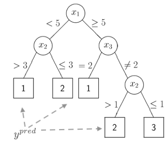
> - **split nodes:** partitioning rules that use one of the input variables
> - **leave nodes:** simple models, usually just the mean of *y*of hte corresponding data subset, this is the end of the tree. ***this is the prediction, ŷ***
>
> *the partitioning is usually binary, which means usually 2 subsets*
### advantages:
- no complex computations: prediction is fast
- don't give “smooth” predictions, you can still approximate smooth surfaces near enough by either using deeper trees or using ensembles of trees
- Tree growing already incorporates feature subset selection because irrelevant features won't be used
### regression tree growin algorithm
init state: we do not have the tree!
1. create the *root* by containing the netire training data
2. compute mean of the `y` for training examples of the node. This is *constant model*
3. compute thte error of *constant model* if it would be the prediction of `y` for the training examples
4. split the data in the middle betweeen each two adjacent values for each feature x.
5. compute how much would SSE reduce because of such patrtitioning this is SSER: ) split the data at the position with biggest reduction.
6. with each new leaf do this from step 1.
### tree pruning
-for this we no longer use simple training error because this will overfit our model
that estimates prediction error we can use either some complexity penalization criterion or error estimation ins separate validation data set
1. for each pair of leaf compute criterion and see whether criterion improve if the subtree would be pruned away and their predecessor would be made in a leaf
2. if would improve do pruning
notes:
- no guarantee in the optimality of the tree
algorithms:
- for classification: ID3, CART, RPART, GUIDE, QUEST
- for rgression:
- ensembles