https://github.com/irfanchahyadi/ml-notes
Complete personal notes for performing Data Analysis, Preprocessing, and Training ML model.
https://github.com/irfanchahyadi/ml-notes
data-analysis machine-learning plotting python
Last synced: about 1 year ago
JSON representation
Complete personal notes for performing Data Analysis, Preprocessing, and Training ML model.
- Host: GitHub
- URL: https://github.com/irfanchahyadi/ml-notes
- Owner: irfanchahyadi
- Created: 2019-06-21T00:48:20.000Z (about 7 years ago)
- Default Branch: master
- Last Pushed: 2020-05-17T08:22:36.000Z (about 6 years ago)
- Last Synced: 2025-04-11T21:22:54.827Z (over 1 year ago)
- Topics: data-analysis, machine-learning, plotting, python
- Language: Python
- Homepage:
- Size: 79.1 KB
- Stars: 4
- Watchers: 0
- Forks: 1
- Open Issues: 0
-
Metadata Files:
- Readme: README.md
Awesome Lists containing this project
README
# ML-Notes
Complete personal notes for performing Data Analysis, Preprocessing, and Training ML model. For easy guideline and quick copy paste snippet to real work. Fit on one page and constantly updated.
## Table of contents
- [Preparation](#Preparation)
- [Importer](#Importer)
- [Input Output](#Input-Output)
- From Other Source : [Flat File](#Flat-File), [SQL](#SQL), [AWS Athena](#AWS-Athena), [GSpread](#GSpread)
- Scraping : [BeautifulSoup](#BeautifulSoup), [Scrapy](#Scrapy)
- [Exploratory Data Analysis](#Exploratory-Data-Analysis)
- [Indexing](#Indexing)
- [Describe](#Describe)
- [Aggregate](#Aggregate)
- [Plotting](#Plotting)
- Relational : [Scatter](#Scatter-plot), [Line](#Line-Plot), [Joint](#Joint-Plot), [Pair](#Pair-Plot), [Regression](#Regression-Plot)
- Distribution : [Pie](#Pie-Plot), [Histogram](#Histogram-Plot), [Bar](#Bar-Plot), [Strip](#Strip-Plot), [Swarm](#Swarm-Plot), [Box](#Box-Plot), [Violin](#Violin-Plot), [Categorical](#Categorical-Plot)
- Other : [Heat Map](#Heat-Map)
- [Properties](#Properties)
- [Preprocessing](#Preprocessing)
- [Feature Engineering](#Feature-Engineering)
- [Missing Value](#Missing-Value)
- [Categorical Feature](#Categorical-Feature)
- [Transform](#Transform)
- [Scaling and Normalize](#Scaling-and-Normalize)
- [Training Model](#Training-Model)
- [Feature Selection](#Feature-Selection)
- [Cross Validation](#Cross-Validation)
- [Train Model](#Train-Model)
- [Evaluation](#Evaluation)
- [Hyperparameter Tuning](#Hyperparameter-Tuning)
- [Pipeline](#Pipeline)
- [Neural Network](#Neural-Network)
- Tensor Flow :
- Keras Model :
- [Build Model](#Build-Keras-Model)
- [Create Callback](#Create-Keras-Callback)
- [Train Model](#Train-Keras-Model)
- [Evaluate Model](#Evaluate-Keras-Model)
- PyTorch :
- [Miscellaneous](#Miscellaneous)
- [Basic Python](#Basic-Python)
- [Regex Cheatsheet](#Regex-Cheatsheet)
- [Datetime Cheatsheet](#Datetime-Cheatsheet)
- [CSS Selector Cheatsheet](#CSS-Selector-Cheatsheet)
- [Matplotlib Cheatsheet](#Matplotlib-Cheatsheet)
## Preparation
### Importer
```python
# Most used
import numpy as np # numerical analysis and matrix computation
import pandas as pd # data manipulation and analysis on tabular data
import matplotlib.pyplot as plt # plotting data
import seaborn as sns # data visualization based on matplotlib
# Connection to data
import pymysql # connect to mysql database
import pyodbc # connect to sql server database
import pyathena # connect to aws athena
import gspread # connect to gspread
from oauth2client.service_account import ServiceAccountCredentials # google auth
from gspread_dataframe import get_as_dataframe, set_with_dataframe # library i/o directly from df
# Scikit-learn
from sklearn.preprocessing import Imputer, scale, StandardScaler
from sklearn.model_selection import train_test_split, cross_val_score, GridSearchCV, RandomizedSearchCV
from sklearn.metrics import mean_squared_error, classification_report, confusion_matrix, roc_curve, roc_auc_score
from sklearn.pipeline import Pipeline
# Scikit-learn Model
from sklearn.neighbors import KNeighborsClassifier
from sklearn.tree import DecisionTreeClassifier
from sklearn.linear_model import LinearRegression, Lasso, Ridge, ElasticNet, LogisticRegression
from sklearn.svm import SVC
# Other Tools
%reload_ext dotenv # reload dotenv on jupyter notebook
%dotenv # load dotenv
import os # os interface, directory, path
import glob # find file on directory with wildcard
import pickle # save/load object on python into/from binary file
import re # find regex pattern on string
import scipy # scientific computing
import statsmodels.api as sm # statistic lib for python
import requests # http for human
from bs4 import BeautifulSoup # tool for scrape web page
```
### Input Output
Create DataFrame from list / dict.
```python
data = [{'name': 'A', 'height': 172, 'weight': 78},
{'name': 'B', 'height': 168, 'weight': 75},
{'name': 'C', 'height': 183, 'weight': 81},
{'name': 'D', 'height': 175, 'weight': 77}]
pd.DataFrame(data) # from list of dict
data = {'name': ['A', 'B', 'C', 'D'],
'height': [172, 168, 183, 175],
'weight': [78, 75, 81, 77]}
pd.DataFrame(data) # from dict
data = [('A', 172, 78),
('B', 168, 75),
('C', 183, 81),
('D', 175, 77)]
columns = ['name', 'height', 'weight']
pd.DataFrame(data, columns=columns) # from records
```
Generate random data.
```python
X = np.random.randn(100, 3) # 100 x 3 random std normal dist array
X = np.random.normal(1, 2, size=(100, 3)) # 100 x 3 random normal with mean 1 and stddev 2
from sklearn.datasets import make_regression, make_classification, make_blobs
# generate 100 row data for regression with 10 feature but only 5 informative
X, y = make_regression(n_samples=100, n_features=10, n_informative=5, noise=0.0, random_state=42)
# generate 100 row data for classification with 10 feature but only 5 informative with 3 classes
X, y = make_classification(n_samples=100, n_features=10, n_informative=5, n_classes=3, random_state=42)
# generate 100 row data for clustering with 10 feature with 3 cluster
X, y = make_blobs(n_samples=100, n_features=10, centers=3, cluster_std=1.0, random_state=42)
```
Load sample data.
```python
from sklearn.datasets import load_boston, load_digits, load_iris
d = load_boston() # load data dict 'like' of numpy.ndarray
df = pd.DataFrame(d.data, columns=d.feature_names) # create dataframe with column name
df['TargetCol'] = d.target # add TargetCol column
```
#### Flat File
```python
df = pd.read_csv('data.csv', sep=',', index_col='col1', na_values='-', parse_dates=True)
df = pd.read_excel('data.xlsx', sheet_name='Sheet1', usecols='A,C,E:F')
```
#### SQL
```python
con = pymysql.connect(user=user, password=pwd, database=db, host=host) # mysql
con = pyodbc.connect('DRIVER={ODBC Driver 11 for SQL Server};
SERVER=server_name;DATABASE=db_name;UID=username;PWD=password') # sql server
con = create_engine('mysql+pymysql://username:password@host/database') # with sqlalchemy.create_engine
query = 'select * from employee where name = %(name)s'
df = pd.read_sql(query, con, params={'name': 'value'}) # qieru or table name
df.to_sql(table_name, con, index=False, if_exists='replace') # if_exists = replace/append
```
#### AWS Athena
```python
conn = pyathena.connect(aws_access_key_id=id, aws_secret_access_key=secret,
s3_staging_dir=stgdir, region_name=region)
query = 'select * from employee'
df = pd.read_sql(query, conn)
```
#### GSpread
```python
scope = ['https://spreadsheets.google.com/feeds','https://www.googleapis.com/auth/drive']
creds = ServiceAccountCredentials.from_json_keyfile_name('client_secret.json', scope)
client = gspread.authorize(creds)
sheet = client.open('FileNameOnGDrive').get_worksheet(0)
df = get_as_dataframe(sheet, usecols=list(range(10))) # use additional gspread_dataframe lib
data = sheet.get_all_values()
header = data.pop(0)
df = pd.DataFrame(data, columns=header) # only use gspread
```
#### BeautifulSoup
```python
HEADERS = {'User-Agent': 'Mozilla/5.0 (Windows NT 10.0; Win64; x64) AppleWebKit/537.36 (KHTML, like Gecko) Chrome/76.0.3809.132 Safari/537.36'}
res = requests.get(url, headers=HEADERS) # request url, with user agent on headers
soup = bs4.BeautifulSoup(res.content, 'html.parser') # create soup object
rows = soup.select('div.product') # selector, see misc
text = soup.select('div.product > a').text # get text of link
href = soup.select('div.product > a')['href'] # get href attribute of link
```
#### Scrapy
```python
# Shell command:
scrapy startproject project_name # create new project
cd project_name
scrapy genspider spider_name url # generate new spider
scrapy crawl spider_name # run spider
scrapy crawl spider_name -o result.csv # run spider, save output as csv
scrapy shell url # testing shell to specific url
# Spider example 1 :
class QuotesSpider(scrapy.Spider):
name = 'quotes'
start_urls = ['http://quotes.toscrape.com']
def parse(self, response):
self.log('I just visited: ' + response.url)
# List of quotes
for quote in response.css('div.quote'):
item = {'author_name': quote.css('small.author::text').extract_first(),
'text': quote.css('span.text::text').extract_first(),
'tags': quote.css('a.tag::text').extract()}
yield item
# Follow pagination link
next_link = response.css('li.next > a::attr(href)').extract_first()
if next_link:
full_next_link = response.urljoin(rel_link)
yield scrapy.Request(url=full_next_link, callback=self.parse)
```
## Exploratory Data Analysis
### Indexing
```python
df.col1 # return series col1, easy way
df['col1'] # return series col1, robust way
df[['col1', 'col2']] # return dataframe consist col1 and col2
df.loc[5:10, ['col1','col2']] # return dataframe from row 5:10 column col1 and col2
df.iloc[5:10, 3:5] # return dataframe from row 5:10 column 3:5
df.head() # return first 5 rows, df.tail() return last 5 rows
df[df.col1 == 'abc'] # filter by comparison, use ==, !=, >, <, >=, <=
df[(df.col1 == 'abc') & (df.col2 > 50)] # conditional filter, use &(and), |(or), ~(not), ^(xor), .any(), .all()
df[df.col1.isna()] # filter by col1 is na
df[df.col1.isnull()] # filter by col1 is null, otherwise use .notnull()
df[df.col1.isin(['a','b'])] # filter by col1 is in list
df[df.col1.between(70, 80)] # filter by col1 value between 2 values
df.filter(regex = 'pattern') # filter by regex pattern, see misc
for idx, row in df.iterrows(): # iterate dataframe by rows
print(row['col1']) # return index and series of row
pd.options.display.max_rows = len(df) # default 60 rows
```
### Describe
```python
df.shape # number of rows and cols
df.columns # columns dataframe
df.index # index dataframe
df.T # transpose dataframe
df.info() # info number of rows and cols, dtype each col, memory size
df.describe(include='all') # statistical descriptive: unique, mean, std, min, max, quartile
df.skew() # degree of symetrical, 0 symmetry, + righthand longer, - lefthand longer
df.kurt() # degree of peakedness, 0 normal dist, + too peaked, - almost flat
df.corr() # correlation matrix
df.isnull().sum() # count null value each column, df.isnull() = df.isna()
df.col1.unique() # return unique value of col1
df.nunique() # unique value each column
df.sample(10) # return random sample 10 rows
df['col1'].value_counts(normalize=True) # frequency each value
df.sort_values(['col1'], ascending=True) # sort by col1 ascending, .sort_index() for index
df.drop_duplicates(subset='col1', keep='first', inplace=True) # drop duplicate based on subset
```
### Aggregate
```python
df.sum() # use sum, count, median, min, mean, var, std, nunique, quantile([0.25,0.75])
df.groupby(['col1']).size() # group by col1
df.groupby(df.col1).TargetCol.agg([np.mean, 'count']) # multi aggregate function on 1 column
df.groupby('col1').agg({'col2': 'count', 'col3': 'mean'}) # multi aggregate function on multi columns
df.pivot(index='col1', columns='col2', values='col3') # reshape to pivot, error when duplicate
df.pivot_table(index='col1', columns='col2', values='col3', aggfunc='sum') # pivot table, like excel
flat = pd.DataFrame(df.to_records()) # flatten multiindex dataframe
```
### Plotting
#### Scatter plot
```python
plt.scatter(x, y, c, s)
# x, y, c, s array like object, c (color) can be color format string, s (size) can be scalar
# also df.plot.scatter(x='col1', y='col2', c='col3', s='col4') or
# sns.scatterplot(x='col1', y='col2', hue='col3', size='col4', style='col5', data=df)
```

#### Line Plot
```python
plt.plot(x, y, 'ro--')
# x and y array like object, 'ro--' means red circle marker with dash line (see matplotlib cheatsheet below)
# also written as plt.plot(x, y, color='r', marker='o', linestyle='--') you can also use df.plot() or
# sns.lineplot(x='col1', y='col2', hue='col3', size='col4', data=df)
```

#### Joint Plot
```python
sns.jointplot(x='col1', y='col2', data=df, kind='reg') # kind = scatter/reg/resid/kde/hex
# Joint 2 two type distrbution plot and kind plot
```

#### Pair Plot
```python
sns.pairplot(df, x_vars=['col1'], y_vars=['col2'], hue='col3', kind='scatter', diag_kind='auto')
# multi joint plot, _vars for filter column, kind = scatter/reg, diag_kind = hist/kde
```

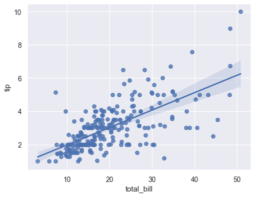
#### Regression Plot
```python
regplot(x='col1', y='col2', data=df, ci=95, order=1)
# scatter plot + regression fit, ci (confidence interval 0-100), order (polynomial order)
```
#### Pie Plot
```python
plt.pie(x, labels, explode, autopct='%1.1f%%')
# x, labels, explode array like also df.plot.pie(y='col1') lable get from index
```

#### Histogram Plot
```python
plt.hist(x, bins=50, density=False, cumulative=False)
# x array like, density (probability density), cumulative probability
# also df.plot.hist('col1') or sns.distplot(x)
```

#### Bar Plot
```python
plt.bar(x, y) # or plt.barh(x, y)
# x array like, also df.plot.bar(x='col1', y=['col2','col3'], stacked=True, subplots=False)
# sns.countplot(x='col1', y='col2', hue='col3', data=df, orient='v')
# sns.barplot(x='col1', y='col2', hue='col3', data=df, orient='v')
```

#### Strip Plot
```python
sns.stripplot(x='col1', y='col2', hue='col3', data=df, jitter=True, dodge=False, orient='v')
# for few data, jitter=True makes point not overwrite on top each other
```

#### Swarm Plot
```python
sns.swarmplot(x='col1', y='col2', hue='col3', data=df, dodge=False, orient='v')
# for few data, more clearly than stripplot, dodge=True makes each cat in hue separable
```

#### Box Plot
```python
sns.boxplot(x='col1', y='col2', hue='col3', data=df, dodge=False, orient='v')
# for large data, include median, Q1 & Q3, IQR (Q3-Q1), min (Q1-1.5*IQR), max (Q3+1.5*IQR) and outliers
```

#### Violin Plot
```python
sns.violinplot(x='col1', y='col2', hue='col3', data=df, dodge=False, orient='v')
# kernel density plot (KDE) for visualize clearly distribution of data
```

#### Categorical Plot
```python
sns.catplot(x='col1', y='col2', hue='col3', data=df, row='col4', col='col5', col_wrap=4,
kind='strip', sharex=True, sharey=True, orient='v')
# categorical plot with facetgrid options
```

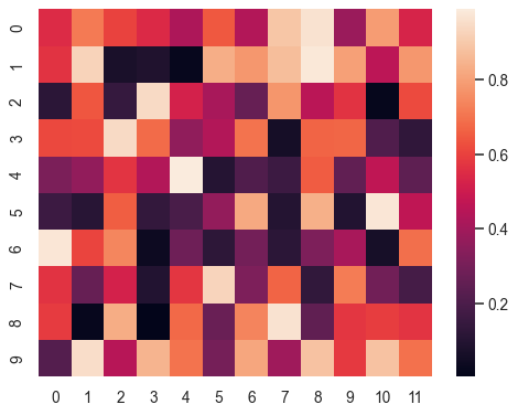
#### Heat Map
```python
sns.heatmap(df.corr(), annot=True, fmt='.2g', annot_kws={'size': 8}, square=True, cmap=plt.cm.Reds)
# useful for plot correlation, annot (write value data), fmt (format value), square, cmap (color map)
# other option use df.corr().style.background_gradient(cmap='coolwarm').set_precision(2)
```
#### Properties
```python
plt.figure(figsize=(15,8))
fig, ax = plt.subplots(1, 2, sharex=False, sharey=False, figsize=(15,4)) # subplots, access with ax[0,1]
plt.title('title') # or ax.set_title
plt.xlabel('foo') # or plt.ylabel, ax.set_xlabel, ax.set_ylabel
plt.xticks(x, labels) # x and labels list, or ax.set_xticks
plt.xticks(rotation=90) # rotate xticks
plt.xlim(0, 100) # or ylim, ax.set_xlim, ax.set_ylim
plt.legend(loc='best') # or ax.legend, loc = upper/lower/right/left/center/upper right
plt.rcParams['figure.figsize'] = (16, 10) # setting default figsize
plt.style.use('classic') # find all style on plt.style.available
g = sns.FacetGrid(df, row='col1', col='col2', hue='col3') # comparable subplot row by col1 col by col2
g.map(plt.hist, 'col4', bins=50) # with histogram count col4
g.map(plt.scatter, 'col4', 'col5') # or with scatter plot col4 and col5
```
## Preprocessing
### Feature Engineering
Basic Operation
```python
df['new_col'] = df.col1 / 1000 # create new column
df = df.drop('col1', axis=1) # drop column
df = df.drop(df[df.col1 == 'abc'].index) # drop row which col1 equal to 'abc'
df.col1 = df.col1.astype(str) # convert column to string, also use 'category', 'int32'
df.col1 = pd.to_numeric(df.col1, error='coerce') # convert column to numeric
df.col1 = pd.to_datetime(df.col1, error='coerce') # convert column to datetime
df.col1 = pd.Categorical(df.col1, categories=['A','B','C'], ordered=True) # convert column to category
df.col1.str[:2] # access string method/properties
df.col1.dt.strftime('%d/%m/%Y') # access datetime method/properties
df.values # convert dataframe to numpy array
```
Map, Apply, Applymap
```python
# Map (Series only)
d = {1: 'one', 2: 'two', 3: 'three'}
df.col1.map(d)
# Apply (Series)
df.col1.apply(func) # element wise
# Apply (Dataframe)
sum_col1, sum_col2 = df[['col1', 'col2']].apply(sum) # apply to axis=0 (row)
df['new_col'] = df.apply(lambda x: x[0] + x[1], axis=1) # apply to axis=1 (column)
# Applymap (Dataframe only)
df.applymap(func) # element wise
# Numpy Vectorize
np.vectorize(func)(A) # element wise
```
### Merge Data
```python
# Append
df1.append(df2, ignore_index=True) # stacked vertical with reset index
# Concat
pd.concat([df1, df2, df3], ignore_index=True) # stacked vertical with reset index, axis=0
# Join
# Merge
df1.merge(df2, on='key_col')
pd.merge(df1, df2, on='key_col', how='inner') # how: left, right, outer, inner
pd.merge(df1, df2, left_on='lkey_col', right_on='rkey_col')
```
### Missing Value
```python
df = df.fillna(0, method=None) # None/backfill/bfill/pad/ffill
imp = Imputer(missing_values='NaN', strategy='mean', axis=0) # strategy = mean/median/most_frequent
imp.fit(X)
X = enc.transform(X) # perform imputing, or use .fit_transform
```
### Categorical Feature
```python
df = pd.get_dummies(df, columns=['col1'], prefix='col1')
enc = LabelBinarizer() # label with value 0 or 1
enc = LabelEncoder() # label with value 0 to n-1
enc = OrdinalEncoder() # label with value 0 to n-1, multi column
enc = OneHotEncoder(handle_unknown='error') # create dummy n column binarize, handle_unknown = error/ignore
enc.fit(X)
X = enc.transform(X) # perform encoding, or use .fit_transform
X = enc.inverse_transform(X) # decode back to original
```
### Transform
```python
```
### Scaling and Normalize
```python
scaler = StandardScaler() # scale data to mean 0 and stddev 1
scaler = MinMaxScaler(feature_range=(0, 1)) # scale data to 0 to 1 (can be set as -1 to 1)
scaler = RobustScaler()quantile_range=(25.0, 75.0) # scale data to robust to outlier
scaler = Normalizer(norm='l2') # normalize data
scaler.fit(X)
X = scaler.transform(X) # perform scaling, or use .fit_transform
X = scaler.inverse_transform(X) # scale back to original
```
## Training Model
### Feature Selection
### Cross Validation
```python
# Train test split
X_train, X_test, y_train, y_test = train_test_split(X, y, test_size = 0.2, random_state=42, stratify=y)
# Train test split with Numpy
np.random.shuffle(data)
border = round(data.shap[0] * 0.7)
train, test = np.split(data, [border])
# Cross Validation
cv = cross_val_score(model, X, y, cv=5, scoring='r2', ) # (Stratified) KFold CV, return list of score
```
### Train Model
```python
# Classification model
clf = LogisticRegression(penalty='l1', C=1.0)
# C inverse regularization, smaller C stronger reg
clf = KNeighborsClassifier(n_neighbors=3)
# n_neighbors number neighbors
clf = DecisionTreeClassifier(max_depth=3, criterion='entropy')
# criterion = gini/entropy, other params: min_sample_split, min_sample_leaf, max_features
```
### Evaluation
```python
accuracy = model.score(X_test, y_test) # get accuracy (depend on model)
```
### Hyperparameter Tuning
```python
# Grid Sarch CV: Try every parameter combination
params = {'C': [1, 0.5, 0.1, 0.05, 0.01]}
grid_cv = GridSearchCV(model, params, cv=5, scoring='r2')
grid_cv.fit(X, y) # print grid_cv.best_params_ and grid_cv.best_score_
# Randomized Search CV: Try every parameter combination based on random distribution
params = {'C': scipy.stats.randint(0, 1)}
randomsearch_cv = RandomizedSearchCV(model, params, cv=5, scoirng='r2')
randomsearch_cv.fit(X, y) # print grid_cv.best_params_ and grid_cv.best_score_
```
### Pipeline
## Neural Network
### Keras Model
### Build Keras Model
```python
# Model
model = Sequential()
# First Layer
model.add(Dense(20, activation='relu', input_shape=(X_train.shape[1],)))
# Hidden Layer
model.add(Dense(20, activation='relu'))
# Output Layer
model.add(Dense(CLASS, activation='softmax'))
# Compile Model
model.compile(loss='categorical_crossentropy', optimizer='Adam', metrics=['accuracy'])
# loss = categorical_crossentropy, mean_squared_error
# optimizer = sgd, adam
# Model Summary
model.summary()
```
### Create Keras Callback
```python
callback = [ReduceLROnPlateau(patience=5), # reduce learning rate when metrics stop improving
EarlyStopping(patience=5), # stop training when metrics stop improving
ModelCheckpoint(filepath='best_model.h5', save_best_only=True)] # save model every period
```
### Train Keras Model
```python
history = model.fit(X_train, y_train, epochs=100, validation_data=(X_val, y_val), callbacks=callback)
# history.history return dict of every metrics each epoch
```
### Evaluate Keras Model
```python
pred = model.predict(X_val).argmax(axis=1) # multiple prediction
pred = model.predict(X_train[0, :].reshape(1, col_shape)).argmax() # single prediction (first sample)
score = round(model.evaluate(X_train, y_train)[1]*100, 2) # metric score
```
## Miscellaneous
### Basic Python
#### Basic data type
Math
```python
np.ceil(5.7) # return 6.0
np.floor(5.7) # return 5.0
np.round(5.7) # return 6.0
round(5.7) # return 6
s.min()
s.max()
```
String
```python
s.isalnum() # return True if alphabetic or numeric
s.isnumeric() # return True if numeric
s.isalpha() # return True if alphabetic
'abc' in s # return True if 'abc' found in s, otherwise use not in
s.find('abc') # return index where substring 'abc' found in s
'abcd: {}'.format(x) # replace {} with value of x, use {:,} for thousand separator, {:.2%} for 2 decimal
s.strip() # return removed leading and trailing space, also use lstrip() or rstrip()
'1,2,3'.split(',') # return list of ['1', '2', '3']
','.join(['a', 'b', 'c']) # join string, return 'a,b,c'
```
List, Tuple & Set
```python
s = [1,2,3,4] # or use list(1,2,3,4)
1 in s # return True if 1 found s
s1 + s2 # concate s1 and s2
s[1] # second item in s
s[1:5] # slice s from 1 to 5 (4 element)
s[1:5:-1] # slice s from 1 to 5 backwards
s.index(3) # return index of 3 in s
s.append(3) # append 3 to end of s
s.reverse() # reverse s, not return anything, or use list(reversed(a))
s.sort() # sort s asc, not return anything, or use sorted(s)
s = (1,2,3,4) # create tuple, immutable list, or use tuple(1,2,3,4)
s = set(1,2,3,4) # create set, unique list
list(map(lambda x: x*2, b)) # map list
list(filter(lambda x: x>2, a)) # filter list
for idx, val in enumerate(s): # iterate over list with index
print(idx, val)
```
Dictionary
```python
d = {'a': 1, 'b': 2, 'c': 3} # or use dict(a=1,b=2,c=3)
d.keys() # return all keys, or use list(d)
d.values() # return all values
'a' in d # return True if 'a' is key in d
d['a'] # get value with keys='a'
del d['a'] # remove item with keys='a'
for key, val in d.items(): # iterate over dict
print(key, val)
```
Numpy.Array
```python
a = np.array([[1,2],[3,4]]) # create array 2x2
```
#### Pickle
```python
try: # check if there is pickle file
with open('data.pickle', 'rb') as f: # open pickle file
data = pickle.load(f) # load data from pickle
except FileNotFoundError: # if pickle file not found
data = some_process() # run some process to get data
with open('data.pickle', 'wb') as f: # create new blank pickle file
pickle.dump(data, f) # save data to pickle
```
#### Others
```python
os.listdir() # get all filename on current directory
```
### Regex Cheatsheet
```
# Cheatsheet:
\d # any number
\D # anything but number
\w # any character
\W # anything but character
. # any character except newline
\b # whitespace
\. # dot character
+ # match 1 or more, use +? for non-greedy
* # match 0 or more, use *? for non-greedy
? # match 0 or 1
^ # start string
$ # end string
() # capturing group, use (?:) for non-capturing group
{} # expect 1-3, ex \d{3} expect 3 digit number, \d{1,3} expect 1-3 digit number
[] # range, ex [A-Z] all capital letter, [abcd] letter a, b, c, d, [^abc] letter NOT a, b, c
| # either or, ex \d{1,4}|[A-z]{4,10} expect 1-4 digit number or 4-10 character word
\n # newline
\s # space
\t # tab
\e # escape
\r # return
# Sample:
'Chapter\s\d{1,4}[\,\.]?\d{0,1}' # get: Chapter 1, Chapter 23, Chapter 649, Chapter 120.5, Chapter 120,5
'[a-zA-Z0-9.]+@[a-zA-Z0-9-]+\.\w+' # get email address
# Usage:
re.findall(r"\w+ly", text) # return ['carefully', 'quickly']
phone = re.sub("[a-zA-Z '()+-]", '', phone) # substitute character with ''
```
### Datetime Cheatsheet
```python
# Cheatsheet:
%Y # Year 4 digit, ex: 1992, 2008, 2014
%y # Year 2 digit, ex: 92, 08, 14
%m # Month 2 digit, ex: 01, 02, ..., 12
%b # Month abbreviation, ex: Jan, Feb, ..., Dec
%B # Month full, ex: January, February, ..., December
%d # Day 2 digit, ex: 01, 02, ..., 31
%w # Weekday 1 digit, ex: 0 (Sunday), 1, ..., 6
%a # Weekday abbreviation, ex: Sun, Mon, ..., Sat
%A # Weekday full, ex: Sunday, Monday, ..., Saturday
%H # Hour (24), ex: 01, 02, ..., 23, 00
%I # Hour (12), ex: 01, 02, ..., 11, 12
%M # Minute, ex: 00, 01, ..., 59
%S # Second, ex: 00, 01, ..., 59
%f # Microsecond, ex: 000000, 000001, ..., 999999
%c # Local datetime representation, ex: Tue Aug 16 21:30:00 1988
%x # Local date representation, ex: 08/16/88
%X # Local time representation, ex: 21:30:00
# Sample:
'%d-%m-%Y %H:%M:%S' # Personal preferred datetime, ex: 16-08-1988 21:30:00
# Usage:
cur_date = datetime.datetime.now() # return current datetime
cur_date.strftime('%d/%m/%Y') # convert datetime object to string
datetime.datetime.strptime('16/08/1988', '%d/%m%Y') # convert string to object
datetime.datetime.fromtimestamp(1575278092) # convert timestamp datetime to datetime
```
### CSS Selector Cheatsheet
```python
# Cheatsheet:
div # div
#abc # id abc
.abc # class abc
div.abc # div with class abc
div.abc.def # div with class both abc and def
div a # a inside div
div > a # a directly inside div
div + p # p immediately after div
div ~ p # p after div
a[target=_blank] # a with attribute target="_blank"
div[style*="border:1px"] # div with style contain "border:1px"
div[style^="border:1px"] # div with style begin with "border:1px"
div[style$="border:1px"] # div with style end with "border:1px"
# Usage:
links = soup.select('div.abc > a')
for link in links:
print(link['href'])
```
### Matplotlib Cheatsheet
```python
# Line Styles Cheatsheet:
- # solid line
-- # dashed line
-. # dash-dot line
: # dotted line
# Marker Styles Cheatsheet:
. # point
o # circle
^ # triangle up, also v, <, >
s # square
p # pentagon
* # star
+ # plus
x # x
| # v line
- # h line
# Color Styles Cheatsheet:
b # blue
g # green
r # red
c # cyan
m # magenta
y # yellow
k # black
w # white
# Cmap Cheatsheet:
viridis, plasma, Reds, cool, hot, coolwarm, hsv, Pastel1, Pastel2, Paired, Set1, Set2, Set3
plt.colormaps() # return all possible cmap
# Usage:
plt.plot(x, y, 'go--')
plt.plot(x, y, color='g', marker='o', linestyle='--')
```