https://github.com/jm199504/financial-knowledge-graphs
小型金融知识图谱构建流程(neo4j / python / cypher / KG)
https://github.com/jm199504/financial-knowledge-graphs
cypher data-analysis graph-database neo4j python
Last synced: about 1 year ago
JSON representation
小型金融知识图谱构建流程(neo4j / python / cypher / KG)
- Host: GitHub
- URL: https://github.com/jm199504/financial-knowledge-graphs
- Owner: jm199504
- Created: 2019-06-27T01:39:14.000Z (about 7 years ago)
- Default Branch: master
- Last Pushed: 2024-07-07T12:38:04.000Z (about 2 years ago)
- Last Synced: 2025-04-11T14:16:55.838Z (over 1 year ago)
- Topics: cypher, data-analysis, graph-database, neo4j, python
- Language: Jupyter Notebook
- Homepage:
- Size: 17.4 MB
- Stars: 2,891
- Watchers: 63
- Forks: 543
- Open Issues: 10
-
Metadata Files:
- Readme: README.md
Awesome Lists containing this project
README
## 小型金融知识图谱构建示例


- [1. 知识图谱存储方式](#1-知识图谱存储方式)
- [1.1 资源描述框架特性](#11-资源描述框架特性)
- [1.2 图数据库特性](#12-图数据库特性)
- [2. 图数据库neo4j](#2-图数据库neo4j)
- [2.1 软件下载](#21-软件下载)
- [2.2 启动登录](#22-启动登录)
- [2.2.1 Windows](#221-windows)
- [2.2.2 MacOS](#222-macos)
- [2.3 储备知识](#23-储备知识)
- [2.4 Windows安装时可能遇到问题及解决方法](#24-windows安装时可能遇到问题及解决方法)
- [3. 知识图谱数据准备](#3-知识图谱数据准备)
- [3.1 免费开源金融数据接口](#31-免费开源金融数据接口)
- [3.1.1 Tushare](#311-tushare)
- [3.1.2 JointQuant](#312-jointquant)
- [3.1.3 导入模块](#313-导入模块)
- [3.2 数据预处理](#32-数据预处理)
- [3.2.1 股票基本信息](#321-股票基本信息)
- [3.2.2 股票持有股东信息](#322-股票持有股东信息)
- [3.2.3 股票概念信息](#323-股票概念信息)
- [3.2.4 股票公告信息](#324-股票公告信息)
- [3.2.5 财经新闻信息](#325-财经新闻信息)
- [3.2.6 概念信息](#326-概念信息)
- [3.2.7 沪股通和深股通成分信息](#327-沪股通和深股通成分信息)
- [3.2.8 股票价格信息](#328-股票价格信息)
- [3.2.9 使用免费接口获取股票数据](#329-使用免费接口获取股票数据)
- [3.3 数据预处理](#33-数据预处理)
- [3.3.1 统计股票的交易日量众数](#331-统计股票的交易日量众数)
- [3.3.2 计算股票对数收益](#332-计算股票对数收益)
- [3.3.3 股票间对数收益率相关系数](#333-股票间对数收益率相关系数)
- [4 搭建金融知识图谱](#4-搭建金融知识图谱)
- [4.1 基于python连接](#41-基于python连接)
- [4.2 读取数据](#42-读取数据)
- [4.3 填充和去重](#43-填充和去重)
- [4.4 创建实体](#44-创建实体)
- [4.5 创建关系](#45-创建关系)
- [5 数据可视化查询](#5-数据可视化查询)
- [5.1 查看所有关联实体](#51-查看所有关联实体)
- [5.2 限制显示数量](#52-限制显示数量)
- [5.3 指定股票间对数收益率相关系数](#53-指定股票间对数收益率相关系数)
- [6 neo4j 图算法](#6-neo4j-图算法)
- [6.1.中心度算法(Centralities)](#61中心度算法centralities)
- [6.2 社区检测算法(Community detection)](#62-社区检测算法community-detection)
- [6.3 路径搜索算法(Path finding)](#63-路径搜索算法path-finding)
- [6.4 相似性算法(Similarity)](#64-相似性算法similarity)
- [6.5 链接预测(Link Prediction)](#65-链接预测link-prediction)
- [6.6 预处理算法(Preprocessing)](#66-预处理算法preprocessing)
- [6.7 算法库安装及导入方法](#67-算法库安装及导入方法)
- [6.8 算法实践——链路预测](#68-算法实践链路预测)
- [6.8.1 Aaamic Adar algorithm](#681-aaamic-adar-algorithm)
- [6.8.2 Common Neighbors](#682-common-neighbors)
- [6.8.3 Resource Allocation](#683-resource-allocation)
- [6.8.4 Total Neighbors](#684-total-neighbors)
## 1. 知识图谱存储方式
知识图谱存储方式主要包含资源描述框架([Resource Description Framework,RDF](https://en.wikipedia.org/wiki/Resource_Description_Framework))和图数据库([Graph Database](https://en.wikipedia.org/wiki/Graph_database))。
### 1.1 资源描述框架特性
- 存储为三元组(Triple)
- 标准的推理引擎
- [W3C标准](https://en.wikipedia.org/wiki/World_Wide_Web_Consortium)
- 易于发布数据
- 多数为学术界场景
### 1.2 图数据库特性
- 节点和关系均可以包含属性
- 没有标准的推理引擎
- 图的遍历效率高
- 事务管理
- 多数为工业界场景
---
## 2. 图数据库neo4j
neo4j是一款[NoSQL](https://en.wikipedia.org/wiki/NoSQL)图数据库,具备高性能的读写可扩展性,基于高效的图形查询语言`Cypher`,更多介绍可访问[neo4j官网](https://neo4j.com/),官网还提供了[Online Sandbox](https://neo4j.com/sandbox/)实现快速上手体验。
### 2.1 软件下载
下载链接:https://neo4j.com/download-center/
### 2.2 启动登录
#### 2.2.1 Windows
- 进入`neo4j`目录
```
cd neo4j/bin
./neo4j start
```
- 启动成功,终端出现如下提示即为启动成功
```
Starting Neo4j.Started neo4j (pid 30914). It is available at http://localhost:7474/ There may be a short delay until the server is ready.
```
(1)访问页面:http://localhost:7474
(2)初始账户和密码均为`neo4j`(`host`类型选择`bolt`)
(3)输入旧密码并输入新密码:启动前注意本地已安装`jdk`(建议安装`jdk version 11`):https://www.oracle.com/java/technologies/javase-downloads.html
#### 2.2.2 MacOS
执行 Add Local DBMS 后,再打开 Neo4j Browser即可
### 2.3 储备知识
在 neo4j 上执行 CRUD 时需要使用 Cypher 查询语言。
- [官网文档](https://neo4j.com/developer/cypher/)
- [个人整理的常见Cypher指令](https://github.com/jm199504/Financial-Knowledge-Graphs/tree/master/cypher%20cheetsheet)
### 2.4 Windows安装时可能遇到问题及解决方法
- 问题:完成安装JDK1.8.0_261后,在启动`neo4j`过程中出现了以下问题:
```
Unable to find any JVMs matching version "11"
```
- 解决方案:提示安装`jdk 11 version`,于是下载了`jdk-11.0.8`,`Mac OS`可通过`ls -la /Library/Java/JavaVirtualMachines/`查看已安装的`jdk`及版本信息。
---
## 3. 知识图谱数据准备
### 3.1 免费开源金融数据接口
Tushare免费账号可能无法拉取数据,可参考issues提供的股票数据获取方法: https://github.com/jm199504/Financial-Knowledge-Graphs/issues/2#issuecomment-801732782
#### 3.1.1 Tushare
官网链接:http://www.tushare.org/
#### 3.1.2 JointQuant
官网链接:https://www.joinquant.com/
#### 3.1.3 导入模块
```python
import tushare as ts # 参考Tushare官网提供的安装方式
import csv
import time
import pandas as pd
# 以下pro_api token可能已过期,可自行前往申请或者使用免费版本
pro = ts.pro_api('4340a981b3102106757287c11833fc14e310c4bacf8275f067c9b82d')
```
### 3.2 数据预处理
#### 3.2.1 股票基本信息
```python
stock_basic = pro.stock_basic(list_status='L', fields='ts_code, symbol, name, industry')
# 重命名行,便于后面导入neo4j
basic_rename = {'ts_code': 'TS代码', 'symbol': '股票代码', 'name': '股票名称', 'industry': '行业'}
stock_basic.rename(columns=basic_rename, inplace=True)
# 保存为stock_basic.csv
stock_basic.to_csv('financial_data\\stock_basic.csv', encoding='gbk')
```
| TS代码 | 股票代码 | 股票名称 | 行业 |
|-----------|----------|------------|----------|
| 000001.SZ | 000001 | 平安银行 | 银行 |
| 000002.SZ | 000002 | 万科A | 全国地产 |
| 000004.SZ | 000004 | 国华网安 | 软件服务 |
| 000005.SZ | 000005 | ST星源 | 环境保护 |
| 000006.SZ | 000006 | 深振业A | 区域地产 |
#### 3.2.2 股票持有股东信息
```python
holders = pd.DataFrame(columns=('ts_code', 'ann_date', 'end_date', 'holder_name', 'hold_amount', 'hold_ratio'))
# 获取一年内所有上市股票股东信息(可以获取一个报告期的)
for i in range(3610):
code = stock_basic['TS代码'].values[i]
holders = pro.top10_holders(ts_code=code, start_date='20180101', end_date='20181231')
holders = holders.append(holders)
if i % 600 == 0:
print(i)
time.sleep(0.4)# 数据接口限制
# 保存为stock_holders.csv
holders.to_csv('financial_data\\stock_holders.csv', encoding='gbk')
holders = pro.holders(ts_code='000001.SZ', start_date='20180101', end_date='20181231')
```
| ts_code | ann_date | end_date | holder_name | hold_amount | hold_ratio |
|-----------|----------|----------|---------------------------------------------------------|---------------|------------|
| 000001.SZ | 20200421 | 20200331 | 中国平安保险(集团)股份有限公司-集团本级-自有资金 | 9.618540e+09 | 49.56 |
| 000001.SZ | 20200421 | 20200331 | 香港中央结算有限公司(陆股通) | 1.669875e+09 | 8.60 |
| 000001.SZ | 20200421 | 20200331 | 中国平安人寿保险股份有限公司-自有资金 | 1.186100e+09 | 6.11 |
| 000001.SZ | 20200421 | 20200331 | 中国平安人寿保险股份有限公司-传统-普通保险产品 | 4.404787e+08 | 2.27 |
| 000001.SZ | 20200421 | 20200331 | 中国证券金融股份有限公司 | 4.292327e+08 | 2.21 |
#### 3.2.3 股票概念信息
```python
concept_details = pd.DataFrame(columns=('id', 'concept_name', 'ts_code', 'name'))
for i in range(358):
id = 'TS' + str(i)
concept_detail = pro.concept_detail(id=id)
concept_details = concept_details.append(concept_detail)
time.sleep(0.4)
# 保存为concept_detail.csv
concept_details.to_csv('financial_data\\stock_concept.csv', encoding='gbk')
```
| id | concept_name | ts_code | name |
|----|---------|----------|--------------|
| TS0 | 密集调研 | 000917.SZ | 电广传媒 |
| TS0 | 密集调研 | 002123.SZ | 梦网集团 |
| TS0 | 密集调研 | 002127.SZ | 南极电商 |
| TS0 | 密集调研 | 002371.SZ | 北方华创 |
| TS0 | 密集调研 | 002460.SZ | 赣锋锂业 |
#### 3.2.4 股票公告信息
```python
for i in range(3610):
code = stock_basic['TS代码'].values[i]
notices = pro.anns(ts_code=code, start_date='20180101', end_date='20181231', year='2018')
notices.to_csv("financial_data\\notices\\"+str(code)+".csv",encoding='utf_8_sig',index=False)
notices = pro.anns(ts_code='000001.SZ', start_date='20180101', end_date='20181231', year='2018')
```
| ts_code | ann_date | title | content |
|-----------|-----------|---------------------------------------------------------------------------------------------|---------------------------------------------|
| 000001.SZ | 20181227 | 关于公开发行A股可转换公司债券申请获得中国证监会核准批复的公告 | 证券代码:000001 证券简称:平安银行 |
| 000001.SZ | 20181226 | 董事会决议公告 | 证券代码:000001 证券简称:平安银行 ... |
| 000001.SZ | 20181219 | 关于成功发行350亿元金融债券的公告 | 证券代码:000001 证券简称:平安银行. |
| 000001.SZ | 20181218 | 关于公开发行A股可转换公司债券申请获中国证监会发行审核委员会南核通过的公告 | 证券代码:000001 证券简称:平安银行 ... |
| 000001.SZ | 20181208 | 关于发行金融债券获准的公告 | 证券代码:000001 证券简称:平安银行⋯ |
#### 3.2.5 财经新闻信息
```python
news = pro.news(src='sina', start_date='20180101', end_date='20181231')
news.to_csv("financial_data\\news.csv",encoding='utf_8_sig')
```
| datetime | content | title |
|---------------------|----------------------------------------------------------------------------------------------|---------------------------------------------------------------------------------------------|
| 2018-11-22 10:09:00 | 【北京:10月末非金融企业贷款增速创历史同期新高 】据中国人民银行营业管理部11月22日披露... | |
| 2018-11-22 10:08:29 | 【湖北省积极推动企业向科创板靠拢,年底将向上交所推荐一批优质企业】湖北省上市指导中心相关人士... | |
| 2018-11-22 10:08:04 | 【上海:加快专利审查速度 进一步缩短专利授权周期】上海市人民政府发布关于加快本市高新技术企业... | |
| 2018-11-22 10:04:35 | 【生意社:稀土价格走势或将上涨】11月20日稀土指数为344点,与上一日持平,较2011年1... | |
| 2018-11-22 10:03:40 | 【上海:加快建设具有全球影响力的科技创新中心 做大做强高新技术产业】上海市人民政府发布关于加... | |
#### 3.2.6 概念信息
```python
concept = pro.concept()
concept.to_csv('financial_data\\concept.csv', encoding='gbk')
```
| code | name | src |
|--------|--------------|--------------|
| TS0 | TSO 密集调研 | ts |
| TS1 | TS1 南北船合并 ts | ts |
| TS2 | TS25G | ts |
| TS3 | TS3 机场 | ts |
| TS4 | TS4 高价股 | ts |
#### 3.2.7 沪股通和深股通成分信息
```python
#获取沪股通成分
sh = pro.hs_const(hs_type='SH')
sh.to_csv("financial_data\\sh.csv",index=False)
#获取深股通成分
sz = pro.hs_const(hs_type='SZ')
sz.to_csv("financial_data\\sz.csv",index=False)
```
| ts_code | hs_type | in_date | out_date | is_new |
|-----------|---------|-----------|----------|--------|
| 601628.SH | SH | 20141117 | None | 1 |
| 601099.SH | SH | 20141117 | None | 1 |
| 601808.SH | SH | 20141117 | None | 1 |
| 601107.SH | SH | 20141117 | None | 1 |
| 601880.SH | SH | 20141117 | None | 1 |
#### 3.2.8 股票价格信息
```python
for i in range(3610):
code = stock_basic['TS代码'].values[i]
price = pro.query('daily', ts_code=code, start_date='20180101', end_date='20181231')
price.to_csv("financial_data\\price\\"+str(code)+".csv",index=False)
```
| ts_code | trade_date | open | high | low | close | pre_close | change | pct_chg | vol | amount |
|-----------|------------|-------|-------|-------|-------|-----------|--------|---------|------------|--------------|
| 000001.SZ | 20200123 | 15.92 | 15.92 | 15.39 | 15.54 | 16.09 | -0.55 | -3.4183 | 1100592.07 | 1723394.336 |
| 000001.SZ | 20200122 | 15.92 | 16.16 | 15.71 | 16.09 | 16.00 | 0.09 | 0.5625 | 719464.91 | 1150933.398 |
| 000001.SZ | 20200121 | 16.34 | 16.34 | 15.93 | 16.00 | 16.45 | -0.45 | -2.7356 | 896603.10 | 1442171.431 |
| 000001.SZ | 20200120 | 16.43 | 16.61 | 16.35 | 16.45 | 16.39 | 0.06 | 0.3661 | 746074.75 | 1226464.649 |
| 000001.SZ | 20200117 | 16.38 | 16.55 | 16.35 | 16.39 | 16.33 | 0.06 | 0.3674 | 605436.69 | 995909.007 |
#### 3.2.9 使用免费接口获取股票数据
```python
import tushare as ts
# 基本面信息
df = ts.get_stock_basics()
# 公告信息
ts.get_notices("000001")
# 新浪股吧
ts.guba_sina()
# 历史价格数据
ts.get_hist_data("000001")
# 历史价格数据(周粒度)
ts.get_hist_data("000001",ktype="w")
# 历史价格数据(1分钟粒度)
ts.get_hist_data("000001",ktype="m")
# 历史价格数据(5分钟粒度)
ts.get_hist_data("000001",ktype="5")
```
#### 3.2.10 指数数据
- sh上证指数
- sz深圳成指
- hs300沪深300
- sz50上证50
- zxb中小板指数
- cyb创业板指数
```
ts.get_hist_data("cyb").head()
```
| date | open | high | close | low | volume | price_change | p_change | ma5 | ma10 | ma20 | v_ma5 | v_ma10 | v_ma20 |
|------------|--------|--------|--------|--------|-------------|--------------|----------|----------|----------|----------|-------------|-------------|--------------|
| 2019-06-19 | 1501.25| 1504.41| 1469.99| 1469.59| 16878786.0 | 14.24 | 0.98 | 1460.376 | 1456.171 | 1466.724 | 13305159.8 | 13847384.5 | 14209395.85 |
| 2019-06-18 | 1443.65| 1460.19| 1455.75| 1437.04| 9075484.0 | 13.40 | 0.93 | 1461.158 | 1454.799 | 1467.911 | 12853513.4 | 13402555.2 | 14119367.10 |
| 2019-06-17 | 1450.56| 1459.21| 1442.35| 1437.14| 9968822.0 | -11.61 | -0.80 | 1467.478 | 1456.122 | 1468.589 | 14905515.8 | 13928269.9 | 14493830.70 |
| 2019-06-14 | 1478.53| 1489.47| 1453.96| 1451.66| 16016380.0 | -25.87 | -1.75 | 1465.276 | 1460.253 | 1470.409 | 15363326.0 | 14201386.5 | 14961172.10 |
| 2019-06-13 | 1474.55| 1485.72| 1479.83| 1464.84| 14586327.0 | 5.93 | 0.40 | 1457.696 | 1463.381 | 1474.394 | 14821981.6 | 13946315.2 | 14942959.45 |
#### 3.2.11 宏观数据(居民消费指数)
```
ts.get_cpi()
```
| month | cpi |
|--------|--------|
| 2019.5 | 102.74 |
| 2019.4 | 102.54 |
| 2019.3 | 102.28 |
| 2019.2 | 101.49 |
| 2019.1 | 101.74 |
#### 3.2.12 获取分笔数据
```python
ts.get_tick_data('000001', date='2018-10-08', src='tt')
```
| time | price | change | volume | amount | type |
|---------|-------|--------|--------|----------|-------|
| 09:25:04| 10.70 | -0.35 | 36779 | 39353530 | 卖盘 |
| 09:30:04| 10.69 | -0.01 | 25165 | 26872673 | 卖盘 |
| 09:30:06| 10.69 | 0.00 | 11092 | 11853208 | 买盘 |
| 09:30:09| 10.68 | -0.01 | 2005 | 2142749 | 卖盘 |
| 09:30:13| 10.68 | 0.00 | 5973 | 6363516 | 买盘 |
#### 3.2.13 价格走势图
```python
from pyecharts.charts import Line
from pyecharts import options as opts
import numpy as np
price = pro.query('daily', ts_code='000001.SZ', start_date='20180101', end_date='20181231')
(
Line()
.add_xaxis(xaxis_data=list(price['trade_date'])[::-1])
.add_yaxis(series_name="close price",y_axis=list(price['close'])[::-1],symbol="circle")
.add_yaxis(series_name="open price",y_axis=list(price['open'])[::-1],symbol="circle")
.add_yaxis(series_name="high price",y_axis=list(price['high'])[::-1],symbol="circle")
.add_yaxis(series_name="low price",y_axis=list(price['low'])[::-1],symbol="circle")
.set_global_opts(title_opts=opts.TitleOpts(title="价格走势图"))
.render_notebook()
)
```
### 3.3 数据预处理
#### 3.3.1 统计股票的交易日量众数
```python
import numpy as np
yaxis = list()
for i in listdir:
stock = pd.read_csv("financial_data\\price_logreturn\\"+i)
yaxis.append(len(stock['logreturn']))
counts = np.bincount(yaxis)
np.argmax(counts)
```
#### 3.3.2 计算股票对数收益
股票对数收益及皮尔逊相关系数的计算公式:

```python
import pandas as pd
import numpy as np
import os
import math
listdir = os.listdir("financial_data\\price")
for l in listdir:
stock = pd.read_csv('financial_data\\price\\'+l)
stock['index'] = [1]* len(stock['close'])
stock['next_close'] = stock.groupby('index')['close'].shift(-1)
stock = stock.drop(index=stock.index[-1])
logreturn = list()
for i in stock.index:
logreturn.append(math.log(stock['next_close'][i]/stock['close'][i]))
stock['logreturn'] = logreturn
stock.to_csv("financial_data\\price_logreturn\\"+l,index=False)
```
#### 3.3.3 股票间对数收益率相关系数
```python
from math import sqrt
def multipl(a,b):
sumofab=0.0
for i in range(len(a)):
temp=a[i]*b[i]
sumofab+=temp
return sumofab
def corrcoef(x,y):
n=len(x)
#求和
sum1=sum(x)
sum2=sum(y)
#求乘积之和
sumofxy=multipl(x,y)
#求平方和
sumofx2 = sum([pow(i,2) for i in x])
sumofy2 = sum([pow(j,2) for j in y])
num=sumofxy-(float(sum1)*float(sum2)/n)
#计算皮尔逊相关系数
den=sqrt((sumofx2-float(sum1**2)/n)*(sumofy2-float(sum2**2)/n))
return num/den
```
由于原始数据达百万条,为节省计算量仅选取前300个股票进行关联性分析
```python
listdir = os.listdir("financial_data\\300stock_logreturn")
s1 = list()
s2 = list()
corr = list()
for i in listdir:
for j in listdir:
stocka = pd.read_csv("financial_data\\300stock_logreturn\\"+i)
stockb = pd.read_csv("financial_data\\300stock_logreturn\\"+j)
if len(stocka['logreturn']) == 242 and len(stockb['logreturn']) == 242:
s1.append(str(i)[:10])
s2.append(str(j)[:10])
corr.append(corrcoef(stocka['logreturn'],stockb['logreturn']))
print(str(i)[:10],str(j)[:10],corrcoef(stocka['logreturn'],stockb['logreturn']))
corrdf = pd.DataFrame()
corrdf['s1'] = s1
corrdf['s2'] = s2
corrdf['corr'] = corr
corrdf.to_csv("financial_data\\corr.csv")
```
### 3.4 文本数据词云及情绪分析
#### 3.4.1 获取数据
```python
#金融量化分析常用到的有:pandas(数据结构)、
#numpy(数组)、matplotlib(可视化)、scipy(统计)
import tushare as ts
import pandas as pd
import matplotlib.pyplot as plt
%matplotlib inline
import jieba
import jieba.analyse
from wordcloud import WordCloud, STOPWORDS, ImageColorGenerator
# 正常显示画图时出现的中文和负号
from pylab import mpl
mpl.rcParams['font.sans-serif']=['SimHei']
mpl.rcParams['axes.unicode_minus']=False
ts.set_token('4340a981b3102106757287c11833fc14e310c4bacf8275f067c9b82d')
pro = ts.pro_api()
df = pro.news(src='sina', start_date='20190601', end_date='20190624')
#获取当前即时财经新闻(如本文是2018年11月17日)
# 数据清洗,保留需要的字段
df=df[['datetime','title','content']]
# 保存数据
df.to_csv("latest_news.csv",encoding="utf_8_sig")
# 查看前5条数据
df.head()
```
#### 3.4.2 财经新闻标题词云
```python
#提取新闻标题内容并转化为列表(list)
#注意原来是pandas的数据格式
mylist = list(df.content.values)
#对内容进行分词(即切割为一个个关键词)
word_list = [" ".join(jieba.cut(sentence)) for sentence in mylist]
new_text = ' '.join(word_list)
#读取图
img = plt.imread("black.jpg")
#设置词云格式
wc = WordCloud(background_color="white",
mask=img,#设置背景图片
max_font_size=120, #字体最大值
random_state=42, #颜色随机性
font_path="c:\windows\fonts\simsun.ttc")
#font_path显示中文字体,使用黑体
#生成词云
wc.generate(new_text)
image_colors = ImageColorGenerator(img)
#设置图片大小
plt.figure(figsize=(14,12))
plt.imshow(wc)
plt.title('财经新闻标题词云\n',fontsize=18)
plt.axis("off")
plt.show()
#将图片保存到本地
# wc.to_file("财经新闻标题词云.jpg")
```

#### 3.4.3 数据清洗(黑名单/固定词)
```python
#数据清洗
#将titles列专门提取出来,并转化为列表形式
d=list(df.content[0])
content=''.join(d)
print(content)
#设置分词黑名单
blacklist = ['个','文本','界面','21','23']
#将某些固定词汇加入分词
stopwords=['产融对接项目','国际金融交易·博览会']
for word in stopwords:
jieba.add_word(word)
#设置blacklist黑名单过滤无关词语
d = {} #将词语转入字典
for word in jieba.cut(content):
if word in blacklist:
continue
if len(word)<2: #去除单个字的词语
continue
d[word] = d.get(word, 0) + 1
#使用jieba.analyse
d=''.join(d)
tags=jieba.analyse.extract_tags(d,topK=100,withWeight=True)
tf=dict((a[0],a[1]) for a in tags)
backgroud_Image = plt.imread('black.jpg')
wc = WordCloud(
background_color='white',
# 设置背景颜色
mask=backgroud_Image,
# 设置背景图片
font_path="c:\windows\fonts\simsun.ttc",
# 若是有中文的话,这句代码必须添加
max_words=10, # 设置最大现实的字数
stopwords=STOPWORDS,# 设置停用词
max_font_size=150,# 设置字体最大值
random_state=30)
wc.generate_from_frequencies(tf)
plt.figure(figsize=(6,6),facecolor='w',edgecolor='k')
plt.imshow(wc)
# 是否显示x轴、y轴下标
plt.title(df.title[0],fontsize=15)
plt.axis('off')
plt.show()
```
#### 3.4.4 情绪分析
```python
from snownlp import SnowNLP
def word_processing(text):
pass
#数据清洗,限于篇幅,代码省略
def sentiment_score_list(dataset):
pass
#数据处理和情绪判断主函数,
#限于篇幅,代码省略
def sentiment_score(senti_text):
s1 = SnowNLP(senti_text)
print(senti_text)
return s1.sentiments
#情绪得分汇总
#将上述新闻标题去掉空格,写入列表里(list)
y=[]
t1=list(df.content)
for i in range(len(t1)):
x=t1[i].split()
x=','.join(x)
if i0:
# p+=1
# else:
# n+=1
# print("正面新闻数目:{0},负面新闻数目:{1}".format(p,n))
```
输出结果:
```
【第八届金交会闭幕,意向签约总额近3500亿元】6月21日至23日,为期三天的第八届中国(广州)国际金融交易·博览会在广州举办。本届金交会上,广东新设机构平台9家,收集48个产融对接项目,意向签约总额近3500亿元,有7个粤港澳大湾区项目是首次集中交换签约文本。深圳证券交易所广州服务基地在本届金交会正式授牌成立,将更好地推动广东省企业上市、发行固定收益产品,支持区域内上市公司做优做强。(界面)
情绪得分: 0.921750008323056
【科创板发行接二连三!睿创微纳、天准科技将于7月2日网上申购】6月23日晚间,记者获悉,睿创微纳和天准科技即将在上交所披露招股意向书、上市发行安排及初步询价公告等多个文件。公告显示,睿创微纳股票代码为688002,网上申购代码为787002。天准科技股票代码为688003,网上申购代码为787003。睿创微纳、天准科技网上、网下申购时间均为7月2日,将于7月4日公布中签结果。(证券时报)
情绪得分: 0.33760371797103894
【东盟峰会主席声明反对贸易保护主义】第34届东盟峰会23日在泰国首都曼谷闭幕。当天公布的本届东盟峰会主席声明说,东盟反对贸易保护主义,支持维护多边贸易体制。(新华社)
情绪得分: 0.05343571003642067
```
### 3.5 数据可视化
#### 3.5.1 获取数据
```python
#先引入后面可能用到的包(package)
import pandas as pd
import numpy as np
import matplotlib.pyplot as plt
#正常显示画图时出现的中文
from pylab import mpl
#这里使用微软雅黑字体
mpl.rcParams['font.sans-serif']=['SimHei']
#画图时显示负号
mpl.rcParams['axes.unicode_minus']=False
import seaborn as sns #画图用的
import tushare as ts
#Jupyter Notebook特有的magic命令
#直接在行内显示图形
%matplotlib inline
sh=ts.get_k_data(code='sh',ktype='D',
autype='qfq', start='1990-12-20')
#code:股票代码,个股主要使用代码,如‘600000’
#ktype:'D':日数据;‘m’:月数据,‘Y’:年数据
#autype:复权选择,默认‘qfq’前复权
#start:起始时间
#end:默认当前时间
#查看下数据前5行
sh.head(5)
```
| date | open | close | high | low | volume | code |
|------------|-------|-------|-------|-------|--------|------|
| 1990-12-20 | 113.1 | 113.5 | 113.5 | 112.85| 1990.0 | sh |
| 1990-12-21 | 113.5 | 113.5 | 113.5 | 113.4 | 1190.0 | sh |
| 1990-12-24 | 113.5 | 114.0 | 114.0 | 113.3 | 8070.0 | sh |
| 1990-12-25 | 114.0 | 114.1 | 114.2 | 114.0 | 2780.0 | sh |
| 1990-12-26 | 114.4 | 114.3 | 114.4 | 114.2 | 310.0 | sh |
#### 3.5.2 绘制收盘价趋势图
```python
#将数据列表中的第0列'date'设置为索引
sh.index=pd.to_datetime(sh.date)
#画出上证指数收盘价的走势
sh['close'].plot(figsize=(12,6))
plt.title('上证指数1990-2018年走势图')
plt.xlabel('日期')
plt.show()
```

#### 3.5.3 描述性统计
```python
#pandas的describe()函数提供了数据的描述性统计
#count:数据样本,mean:均值,std:标准差
sh.describe().round(2)
```
| | open | close | high | low | volume |
|---------|---------|---------|---------|---------|--------------|
| count | 6808.00 | 6808.00 | 6808.00 | 6808.00 | 6.808000e+03 |
| mean | 1957.80 | 1959.08 | 1976.41 | 1937.84 | 7.431684e+07 |
| std | 1074.56 | 1075.94 | 1085.71 | 1062.06 | 1.055240e+08 |
| min | 105.50 | 105.50 | 105.50 | 105.50 | 1.000000e+01 |
| 25% | 1186.85 | 1185.01 | 1194.68 | 1171.79 | 5.272635e+06 |
| 50% | 1831.68 | 1832.42 | 1842.81 | 1813.92 | 2.375030e+07 |
| 75% | 2772.39 | 2779.86 | 2807.02 | 2744.36 | 1.144936e+08 |
| max | 6057.43 | 6092.06 | 6124.04 | 6040.71 | 8.571328e+08 |
#### 3.5.4 绘制每日成交量趋势图
```python
sh.loc["2007-01-01":]["volume"].plot(figsize=(12,6))
plt.title('上证指数2007-2018年日成交量图')
plt.xlabel('日期')
plt.show()
```

#### 3.5.5 绘制均线趋势图
```python
#这里的平均线是通过自定义函数,手动设置20,52,252日均线
#移动平均线:
ma_day = [20,52,252]
for ma in ma_day:
column_name = "%s日均线" %(str(ma))
sh[column_name] =sh["close"].rolling(ma).mean()
#sh.tail(3)
#画出2010年以来收盘价和均线图
sh.loc['2010-10-8':][["close",
"20日均线","52日均线","252日均线"]].plot(figsize=(12,6))
plt.title('2010-2018上证指数走势图')
plt.xlabel('日期')
plt.show()
```

#### 3.5.6 绘制日收益率趋势图
```
#2005年之前的数据噪音太大,主要分析2005年之后的
sh["日收益率"] = sh["close"].pct_change()
sh["日收益率"].loc['2005-01-01':].plot(figsize=(12,4))
plt.xlabel('日期')
plt.ylabel('收益率')
plt.title('2005-2018年上证指数日收益率')
plt.show()
```

#### 3.5.7 分析多股票
```python
#分析下常见的几个股票指数
stocks={'上证指数':'sh','深证指数':'sz','沪深300':'hs300',
'上证50':'sz50','中小板指':'zxb','创业板':'cyb'}
stock_index=pd.DataFrame()
for stock in stocks.values():
stock_index[stock]=ts.get_k_data(stock,ktype='D',
autype='qfq', start='2005-01-01')['close']
#stock_index.head()
#计算这些股票指数每日涨跌幅
tech_rets = stock_index.pct_change()[1:]
print(tech_rets)
#tech_rets.head()
#收益率描述性统计
tech_rets.describe()
#结果不在此报告
#均值其实都大于0
tech_rets.mean()*100 #转换为%
```
| | sh | sz | hs300 | sz50 | zxb | cyb |
|----|-----------|-----------|-----------|-----------|-----------|-----------|
| 1 | 0.007379 | 0.009070 | -0.008002 | 0.005272 | 0.004482 | 0.001279 |
| 2 | -0.009992 | -0.007904 | -0.016797 | -0.010741 | -0.025450 | 0.029334 |
| 3 | 0.004292 | 0.002265 | 0.022683 | 0.001362 | 0.009146 | 0.040661 |
| 4 | 0.006146 | 0.008941 | -0.013917 | 0.011377 | -0.044799 | -0.002164 |
| 5 | 0.004040 | 0.002233 | -0.013060 | 0.005846 | 0.014144 | 0.009998 |
| ...| ... | ... | ... | ... | ... | ... |
| 3524 | 0.001933 | 0.007996 | 0.000000 | 0.002929 | 0.000000 | 0.000000 |
| 3525 | -0.025805 | -0.027207 | 0.000000 | -0.021746 | 0.000000 | 0.000000 |
| 3526 | -0.001749 | 0.001361 | 0.000000 | -0.005508 | 0.000000 | 0.000000 |
| 3527 | -0.004416 | -0.003548 | 0.000000 | -0.000961 | 0.000000 | 0.000000 |
#### 3.5.8 绘制相关系数
```python
# jointplot这个函数可以画出两个指数的”相关性系数“,或者说皮尔森相关系数
sns.jointplot('sh','sz',data=tech_rets)
```

#### 3.5.9 绘制多数据集相关系数
```python
# 成对的比较不同数据集之间的相关性,而对角线则会显示该数据集的直方图
sns.pairplot(tech_rets.iloc[:,3:].dropna())
```

#### 3.5.10 收益率与风险
```python
#构建一个计算股票收益率和标准差的函数
#默认起始时间为'2005-01-01'
def return_risk(stocks,startdate='2005-01-01'):
close=pd.DataFrame()
for stock in stocks.values():
close[stock]=ts.get_k_data(stock,ktype='D',
autype='qfq', start=startdate)['close']
tech_rets = close.pct_change()[1:]
rets = tech_rets.dropna()
ret_mean=rets.mean()*100
ret_std=rets.std()*100
return ret_mean,ret_std
#画图函数
def plot_return_risk():
ret,vol=return_risk(stocks)
color=np.array([ 0.18, 0.96, 0.75, 0.3, 0.9,0.5])
plt.scatter(ret, vol, marker = 'o',
c=color,s = 500,cmap=plt.get_cmap('Spectral'))
plt.xlabel("日收益率均值%")
plt.ylabel("标准差%")
for label,x,y in zip(stocks.keys(),ret,vol):
plt.annotate(label,xy = (x,y),xytext = (20,20),
textcoords = "offset points",
ha = "right",va = "bottom",
bbox = dict(boxstyle = 'round,pad=0.5',
fc = 'yellow', alpha = 0.5),
arrowprops = dict(arrowstyle = "->",
connectionstyle = "arc3,rad=0"))
stocks={'上证指数':'sh','深证指数':'sz','沪深300':'hs300',
'上证50':'sz50','中小板指数':'zxb','创业板指数':'cyb'}
plot_return_risk()
```

```python
stocks={'中国平安':'601318','格力电器':'000651',
'招商银行':'600036','恒生电子':'600570',
'中信证券':'600030','贵州茅台':'600519'}
startdate='2018-01-01'
plot_return_risk()
```

#### 3.5.11 蒙特卡洛模拟
蒙特卡洛模拟是一种统计学方法,用来模拟数据的演变趋势。蒙特卡洛模拟是在二战期间,当时在原子弹研制的项目中,为了模拟裂变物质的中子随机扩散现象,由美国数学家冯·诺伊曼和乌拉姆等发明的一种统计方法。之所以起名叫蒙特卡洛模拟,是因为蒙特卡洛在是欧洲袖珍国家摩纳哥一个城市,这个城市在当时是非常著名的一个赌城。因为赌博的本质是算概率,而蒙特卡洛模拟正是以概率为基础的一种方法,所以用赌城的名字为这种方法命名。蒙特卡洛模拟每次输入都随机选择输入值,通过大量的模拟,最终得出一个累计概率分布图。
```python
df=ts.get_k_data('sh',ktype='D', autype='qfq',
start='2005-01-01')
df.index=pd.to_datetime(df.date)
tech_rets = df.close.pct_change()[1:]
rets = tech_rets.dropna()
#rets.head()
# 结果解释:95%的置信我们每天不会损失超过0.0264...
rets.quantile(0.05)
# -0.02618228439478043
```
#### 3.5.12 蒙特卡洛模拟价格分布图
```python
def monte_carlo(start_price,days,mu,sigma):
dt=1/days
price = np.zeros(days)
price[0] = start_price
shock = np.zeros(days)
drift = np.zeros(days)
for x in range(1,days):
shock[x] = np.random.normal(loc=mu * dt,
scale=sigma * np.sqrt(dt))
drift[x] = mu * dt
price[x] = price[x-1] + (price[x-1] *
(drift[x] + shock[x]))
return price
#模拟次数
runs = 10000
start_price = 2641.34 #今日收盘价
days = 252
mu=rets.mean()
sigma=rets.std()
simulations = np.zeros(runs)
for run in range(runs):
simulations[run] = monte_carlo(start_price,
days,mu,sigma)[days-1]
q = np.percentile(simulations,1)
plt.figure(figsize=(8,6))
plt.hist(simulations,bins=50,color='grey')
plt.figtext(0.6,0.8,s="初始价格: %.2f" % start_price)
plt.figtext(0.6,0.7,"预期价格均值: %.2f" %simulations.mean())
plt.figtext(0.15,0.6,"q(0.99: %.2f)" %q)
plt.axvline(x=q,linewidth=6,color="r")
plt.title("经过 %s 天后上证指数模拟价格分布图" %days,weight="bold")
# Text(0.5,1,'经过 252 天后上证指数模拟价格分布图')
```

#### 3.5.13 借用期权定价里对未来股票走势的假定来进行蒙特卡洛模拟
```python
import numpy as np
from time import time
np.random.seed(2018)
t0=time()
S0=2641.34
T=1.0;
r=0.05;
sigma=rets.std()
M=50;
dt=T/M;
I=250000
S=np.zeros((M+1,I))
S[0]=S0
for t in range(1,M+1):
z=np.random.standard_normal(I)
S[t]=S[t-1]*np.exp((r-0.5*sigma**2)*dt+
sigma*np.sqrt(dt)*z)
s_m=np.sum(S[-1])/I
tnp1=time()-t0
# print('经过250000次模拟,得出1年以后上证指数的预期平均收盘价为:%.2f',%s_m)
# 经过250000次模拟,得出1年以后上证指数的预期平均收盘价为:2776.85
%matplotlib inline
import matplotlib.pyplot as plt
plt.figure(figsize=(10,6))
plt.plot(S[:,:10])
plt.grid(True)
plt.title('上证指数蒙特卡洛模拟其中10条模拟路径图')
plt.xlabel('时间')
plt.ylabel('指数')
plt.show()
```

#### 3.5.16 上证指数蒙特卡洛模拟
```python
plt.figure(figsize=(10,6))
plt.hist(S[-1], bins=120)
plt.grid(True)
plt.xlabel('指数水平')
plt.ylabel('频率')
plt.title('上证指数蒙特卡洛模拟')
# Text(0.5,1,'上证指数蒙特卡洛模拟')
```

## 4 搭建金融知识图谱
安装第三方库
```shell
pip install py2neo
```
### 4.1 基于python连接
具体代码可参考3.1 python操作neo4j-连接
```python
from pandas import DataFrame
from py2neo import Graph,Node,Relationship,NodeMatcher
import pandas as pd
import numpy as np
import os
# 连接Neo4j数据库
graph = Graph('http://localhost:7474/db/data/',username='neo4j',password='neo4j')
```
### 4.2 读取数据
```python
stock = pd.read_csv('stock_basic.csv',encoding="gbk")
holder = pd.read_csv('holders.csv')
concept_num = pd.read_csv('concept.csv')
concept = pd.read_csv('stock_concept.csv')
sh = pd.read_csv('sh.csv')
sz = pd.read_csv('sz.csv')
corr = pd.read_csv('corr.csv')
```
### 4.3 填充和去重
```python
stock['行业'] = stock['行业'].fillna('未知')
holder = holder.drop_duplicates(subset=None, keep='first', inplace=False)
```
### 4.4 创建实体
概念、股票、股东、股通
```python
sz = Node('深股通',名字='深股通')
graph.create(sz)
sh = Node('沪股通',名字='沪股通')
graph.create(sh)
for i in concept_num.values:
a = Node('概念',概念代码=i[1],概念名称=i[2])
print('概念代码:'+str(i[1]),'概念名称:'+str(i[2]))
graph.create(a)
for i in stock.values:
a = Node('股票',TS代码=i[1],股票名称=i[3],行业=i[4])
print('TS代码:'+str(i[1]),'股票名称:'+str(i[3]),'行业:'+str(i[4]))
graph.create(a)
for i in holder.values:
a = Node('股东',TS代码=i[0],股东名称=i[1],持股数量=i[2],持股比例=i[3])
print('TS代码:'+str(i[0]),'股东名称:'+str(i[1]),'持股数量:'+str(i[2]))
graph.create(a)
```

### 4.5 创建关系
股票-股东、股票-概念、股票-公告、股票-股通
```python
matcher = NodeMatcher(graph)
for i in holder.values:
a = matcher.match("股票",TS代码=i[0]).first()
b = matcher.match("股东",TS代码=i[0])
for j in b:
r = Relationship(j,'参股',a)
graph.create(r)
print('TS',str(i[0]))
for i in concept.values:
a = matcher.match("股票",TS代码=i[3]).first()
b = matcher.match("概念",概念代码=i[1]).first()
if a == None or b == None:
continue
r = Relationship(a,'概念属于',b)
graph.create(r)
noticesdir = os.listdir("notices\\")
for n in noticesdir:
notice = pd.read_csv("notices\\"+n,encoding="utf_8_sig")
notice['content'] = notice['content'].fillna('空白')
for i in notice.values:
a = matcher.match("股票",TS代码=i[0]).first()
b = Node('公告',日期=i[1],标题=i[2],内容=i[3])
graph.create(b)
r = Relationship(a,'发布公告',b)
graph.create(r)
print(str(i[0]))
for i in sz.values:
a = matcher.match("股票",TS代码=i[0]).first()
b = matcher.match("深股通").first()
r = Relationship(a,'成分股属于',b)
graph.create(r)
print('TS代码:'+str(i[1]),'--深股通')
for i in sh.values:
a = matcher.match("股票",TS代码=i[0]).first()
b = matcher.match("沪股通").first()
r = Relationship(a,'成分股属于',b)
graph.create(r)
print('TS代码:'+str(i[1]),'--沪股通')
# 构建股票间关联
corr = pd.read_csv("corr.csv")
for i in corr.values:
a = matcher.match("股票",TS代码=i[1][:-1]).first()
b = matcher.match("股票",TS代码=i[2][:-1]).first()
r = Relationship(a,str(i[3]),b)
graph.create(r)
print(i)
```

## 5 数据可视化查询
基于Crypher语言,以平安银行为例进行可视化查询。
### 5.1 查看所有关联实体
```cypher
match p=(m)-[]->(n) where m.股票名称="平安银行" or n.股票名称="平安银行" return p;
```

### 5.2 限制显示数量
计算股票间对数收益率的相关系数后,查看与平安银行股票相关联的实体
```cypher
match p=(m)-[]->(n) where m.股票名称="平安银行" or n.股票名称="平安银行" return p limit 300;
```

### 5.3 指定股票间对数收益率相关系数
```cypher
match p=(m)-[]->(n) where m.股票名称="平安银行" and n.股票名称="万科A" return p;
```

## 6 neo4j 图算法
### 6.1.中心度算法(Centralities)
- [PageRank(页面排名)](https://neo4j.com/docs/graph-algorithms/current/algorithms/page-rank/)
- [ArticleRank(文章排名)](https://neo4j.com/docs/graph-algorithms/current/algorithms/article-rank/)
- [Betweenness Centrality (中介中心度)](https://neo4j.com/docs/graph-algorithms/current/algorithms/betweenness-centrality/)
- [Closeness Centrality (接近中心度)](https://neo4j.com/docs/graph-algorithms/current/algorithms/closeness-centrality/)
- [Harmonic Centrality(谐波中心度)](https://neo4j.com/docs/graph-algorithms/current/algorithms/harmonic-centrality/)
### 6.2 社区检测算法(Community detection)
- [Louvain (鲁汶算法)](https://neo4j.com/docs/graph-data-science/current/algorithms/louvain/)
- [Label Propagation (标签传播)](https://neo4j.com/docs/graph-algorithms/current/algorithms/label-propagation/)
- [Connected Components (连通组件)](https://neo4j.com/docs/graph-algorithms/current/algorithms/connected-components/)
- [Strongly Connected Components (强连通组件)]((https://neo4j.com/docs/graph-algorithms/current/algorithms/strongly-connected-components/)
- [Triangle Counting / Clustering Coefficient (三角计数/聚类系数)](https://neo4j.com/docs/graph-algorithms/current/algorithms/triangle-counting-clustering-coefficient/)
### 6.3 路径搜索算法(Path finding)
- [Minimum Weight Spanning Tree (最小权重生成树)](https://neo4j.com/docs/graph-algorithms/current/algorithms/minimum-weight-spanning-tree/)
- [Shortest Path (最短路径)](https://neo4j.com/docs/graph-algorithms/current/algorithms/shortest-path/)
- [Single Source Shortest Path (单源最短路径)](https://neo4j.com/docs/graph-algorithms/current/algorithms/single-source-shortest-path/)
- [All Pairs Shortest Path (全顶点对最短路径)](https://neo4j.com/docs/graph-algorithms/current/algorithms/all-pairs-shortest-path/)
- [A*(A星)](https://neo4j.com/docs/graph-algorithms/current/algorithms/a_star/)
- [Yen’s K-shortest Paths(Yen-K最短路径)](https://neo4j.com/docs/graph-algorithms/current/algorithms/yen-s-k-shortest-path/)
- [Random Walk (随机游走)](https://neo4j.com/docs/graph-algorithms/current/algorithms/random-walk/)
### 6.4 相似性算法(Similarity)
- [Jaccard Similarity (Jaccard相似度)](https://neo4j.com/docs/graph-algorithms/current/algorithms/similarity-jaccard/)
- [Cosine Similarity (余弦相似度)](https://neo4j.com/docs/graph-algorithms/current/algorithms/similarity-cosine/)
- [Pearson Similarity (Pearson相似度)](https://neo4j.com/docs/graph-algorithms/current/algorithms/similarity-pearson/)
- [Euclidean Distance (欧氏距离)](https://neo4j.com/docs/graph-algorithms/current/algorithms/similarity-euclidean/)
- [Overlap Similarity (重叠相似度)](https://neo4j.com/docs/graph-algorithms/current/algorithms/similarity-overlap/)
### 6.5 链接预测(Link Prediction)
- [Adamic Adar(AA)](https://neo4j.com/docs/graph-algorithms/current/algorithms/linkprediction-adamic-adar/)
- [Common Neighbors(共同近邻)](https://neo4j.com/docs/graph-algorithms/current/algorithms/linkprediction-common-neighbors/)
- [Preferential Attachment(优先连接)](https://neo4j.com/docs/graph-algorithms/current/algorithms/linkprediction-preferential-attachment/)
- [Resource Allocation(资源分配)](https://neo4j.com/docs/graph-algorithms/current/algorithms/linkprediction-resource-allocation/)
- [Same Community(共同社区)](https://neo4j.com/docs/graph-algorithms/current/algorithms/linkprediction-same-community/)
- [Total Neighbors(近邻总数)](https://neo4j.com/docs/graph-algorithms/current/algorithms/linkprediction-total-neighbors/)
### 6.6 预处理算法(Preprocessing)
- [One Hot Encoding(独热编码)](https://neo4j.com/docs/graph-algorithms/current/algorithms/one-hot-encoding/)
### 6.7 算法库安装及导入方法
以Windows OS为例,neo4j的算法库并非在安装包中提供,而需要下载算法包:
(1)下载`graph-algorithms-algo-3.5.4.0.jar`
(2)将`graph-algorithms-algo-3.5.4.0.jar`移动至neo4j数据库根目录下的`plugin`中
(3)修改neo4j数据库目录的`conf`中`neo4j.conf`,添加以下配置
```
dbms.security.procedures.unrestricted=algo.*
```
(4)使用以下命令查看所有算法列表
```cypher
CALL algo.list()
```
### 6.8 算法实践——链路预测
#### 6.8.1 Aaamic Adar algorithm
主要基于判断相邻的两个节点之间的亲密程度作为评判标准,2003年由Lada Adamic 和 Eytan Adar在 [Friends and neighbors on the Web](https://www.sciencedirect.com/science/article/abs/pii/S0378873303000091?via%3Dihub) 提出,其中节点亲密度的计算公式如下:
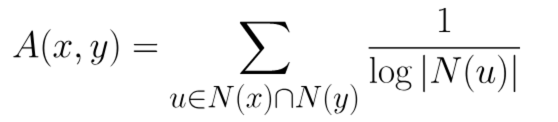
其中`N(u)`表示与节点u相邻的节点集合,若`A(x,y)`表示节点x和节点y不相邻,而该值若越大则紧密度为高。
AAA 算法 cypher 代码参考:
```cypher
MERGE (zhen:Person {name: "Zhen"})
MERGE (praveena:Person {name: "Praveena"})
MERGE (michael:Person {name: "Michael"})
MERGE (arya:Person {name: "Arya"})
MERGE (karin:Person {name: "Karin"})
MERGE (zhen)-[:FRIENDS]-(arya)
MERGE (zhen)-[:FRIENDS]-(praveena)
MERGE (praveena)-[:WORKS_WITH]-(karin)
MERGE (praveena)-[:FRIENDS]-(michael)
MERGE (michael)-[:WORKS_WITH]-(karin)
MERGE (arya)-[:FRIENDS]-(karin)
// 计算 Michael 和 Karin 之间的亲密度
MATCH (p1:Person {name: 'Michael'})
MATCH (p2:Person {name: 'Karin'})
RETURN algo.linkprediction.adamicAdar(p1, p2) AS score
// score: 0.910349
// 基于好友关系计算 Michael 和 Karin 之间的亲密度
MATCH (p1:Person {name: 'Michael'})
MATCH (p2:Person {name: 'Karin'})
RETURN algo.linkprediction.adamicAdar(p1, p2, {relationshipQuery: "FRIENDS"}) AS score
// score: 0.0
```
#### 6.8.2 Common Neighbors
基于节点之间共同近邻数量计算,计算公式如下:

其中N(x)表示与节点x相邻的节点集合,共同近邻表示两个集合的交集,若CN(x,y)值越高,表示节点x和节点y的亲密度越高。
Common Neighbors算法 cypher 代码参考:
```cypher
MATCH (p1:Person {name: 'Michael'})
MATCH (p2:Person {name: 'Karin'})
RETURN algo.linkprediction.commonNeighbors(p1, p2) AS score
```
---
#### 6.8.3 Resource Allocation
资源分配算法,计算公式如下:

其中`N(u)`是与节点`u`相邻的节点集合,RA(x,y)越高表明节点x和节点y的亲密度越大。
Resource Allocation算法 cypher 代码参考:
```cypher
MATCH (p1:Person {name: 'Michael'})
MATCH (p2:Person {name: 'Karin'})
RETURN algo.linkprediction.resourceAllocation(p1, p2) AS score
```
#### 6.8.4 Total Neighbors
指的是相邻节点之间的邻居总数,计算公式如下:

其中`N(u)`是与节点`u`相邻的节点集合。
Total Neighbors算法 cypher 代码参考:
```cypher
MATCH (p1:Person {name: 'Michael'})
MATCH (p2:Person {name: 'Karin'})
RETURN algo.linkprediction.totalNeighbors(p1, p2) AS score
```
官网文档=>链路算法=>介绍:https://neo4j.com/docs/graph-algorithms/3.5/labs-algorithms/linkprediction/