https://github.com/jonasbreuling/scipy_dae
Python implementation of solvers for differential algebraic equation's (DAE's) that should be added to scipy one day.
https://github.com/jonasbreuling/scipy_dae
bdf constraints dae differential-algebraic-equations differential-equations ida implicit implicit-differential-equations navier-stokes-equations ode python radau scipy step-size sundials
Last synced: over 1 year ago
JSON representation
Python implementation of solvers for differential algebraic equation's (DAE's) that should be added to scipy one day.
- Host: GitHub
- URL: https://github.com/jonasbreuling/scipy_dae
- Owner: JonasBreuling
- License: bsd-3-clause
- Created: 2024-02-20T07:32:02.000Z (over 2 years ago)
- Default Branch: main
- Last Pushed: 2025-03-20T07:14:45.000Z (over 1 year ago)
- Last Synced: 2025-04-12T23:36:44.935Z (over 1 year ago)
- Topics: bdf, constraints, dae, differential-algebraic-equations, differential-equations, ida, implicit, implicit-differential-equations, navier-stokes-equations, ode, python, radau, scipy, step-size, sundials
- Language: Python
- Homepage:
- Size: 79.4 MB
- Stars: 25
- Watchers: 5
- Forks: 3
- Open Issues: 7
-
Metadata Files:
- Readme: README.md
- License: LICENSE.txt
Awesome Lists containing this project
README
# scipy_dae - solving differential algebraic equations (DAEs) and implicit differential equations (IDEs) in Python


Python implementation of solvers for differential algebraic equations (DAEs) and implicit differential equations (IDEs) that should be added to scipy one day.
Currently, two different methods are implemented.
* Implicit **Radau IIA** methods of order 2s - 1 with arbitrary number of odd stages.
* Implicit **backward differentiation formula (BDF)** of variable order with quasi-constant step-size and stability/ accuracy enhancement using numerical differentiation formula (NDF).
More information about both methods are given in the specific class documentation.
## To pique your curiosity
The [Kármán vortex street](https://en.wikipedia.org/wiki/K%C3%A1rm%C3%A1n_vortex_street) solved by a finite element discretization of the [weak form of the incompressible Navier-Stokes equations](https://en.wikipedia.org/wiki/Navier%E2%80%93Stokes_equations#Weak_form) using [FEniCS](https://fenicsproject.org/) and the three stage Radau IIA method.
[](https://raw.githubusercontent.com/JonasBreuling/scipy_dae/main/data/img/von_Karman.gif)
## Basic usage
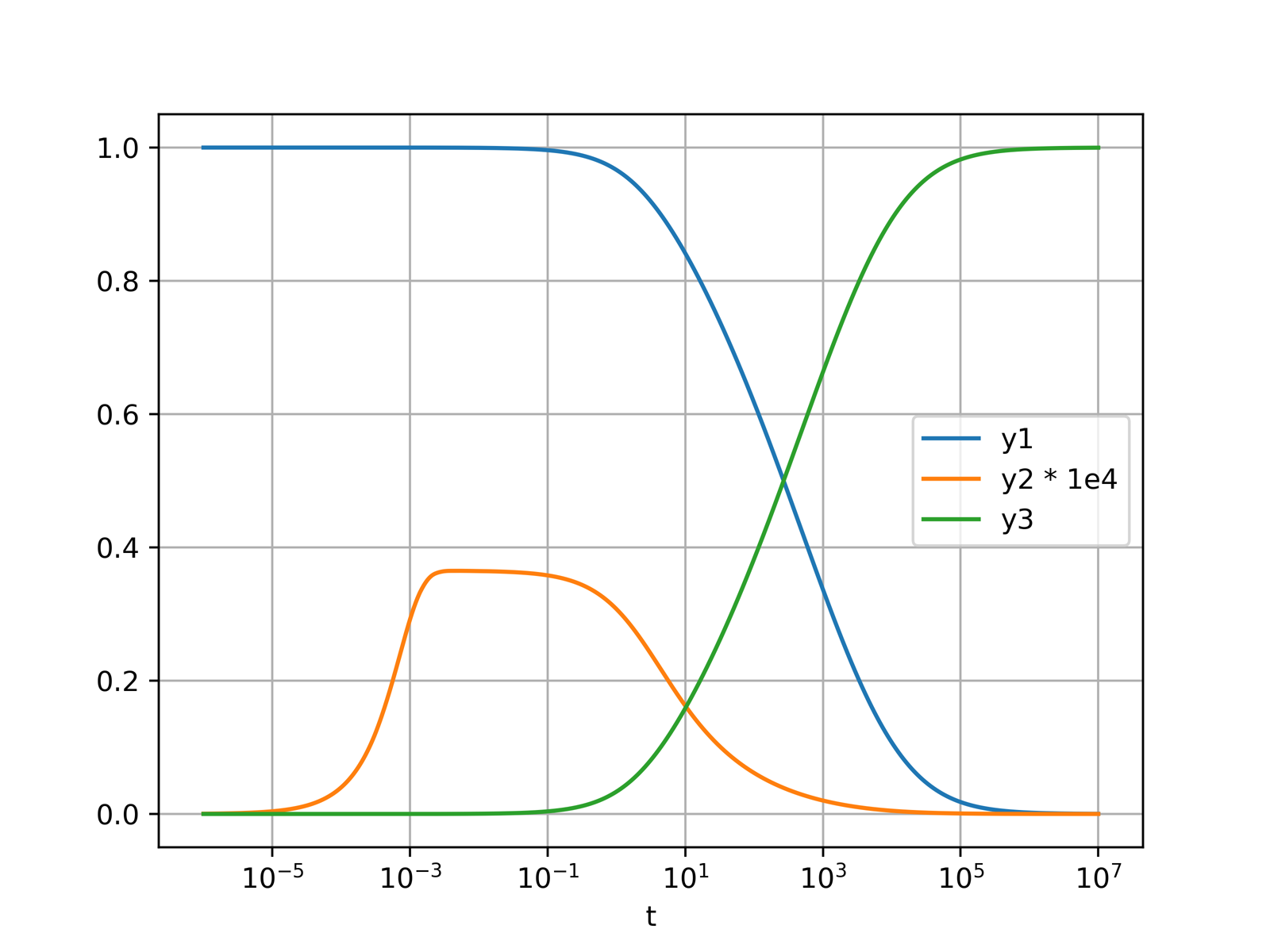
The Robertson problem of semi-stable chemical reaction is a simple system of differential algebraic equations of index 1. It demonstrates the basic usage of the package.
```python
import numpy as np
import matplotlib.pyplot as plt
from scipy_dae.integrate import solve_dae
def F(t, y, yp):
"""Define implicit system of differential algebraic equations."""
y1, y2, y3 = y
y1p, y2p, y3p = yp
F = np.zeros(3, dtype=np.common_type(y, yp))
F[0] = y1p - (-0.04 * y1 + 1e4 * y2 * y3)
F[1] = y2p - (0.04 * y1 - 1e4 * y2 * y3 - 3e7 * y2**2)
F[2] = y1 + y2 + y3 - 1 # algebraic equation
return F
# time span
t0 = 0
t1 = 1e7
t_span = (t0, t1)
t_eval = np.logspace(-6, 7, num=1000)
# initial conditions
y0 = np.array([1, 0, 0], dtype=float)
yp0 = np.array([-0.04, 0.04, 0], dtype=float)
# solver options
method = "Radau"
# method = "BDF" # alternative solver
atol = rtol = 1e-6
# solve DAE system
sol = solve_dae(F, t_span, y0, yp0, atol=atol, rtol=rtol, method=method, t_eval=t_eval)
t = sol.t
y = sol.y
# visualization
fig, ax = plt.subplots()
ax.plot(t, y[0], label="y1")
ax.plot(t, y[1] * 1e4, label="y2 * 1e4")
ax.plot(t, y[2], label="y3")
ax.set_xlabel("t")
ax.set_xscale("log")
ax.legend()
ax.grid()
plt.show()
```
## Advanced usage
More examples are given in the [examples](examples/) directory, which includes
* ordinary differential equations (ODEs)
* [Van der Pol oscillator](examples/odes/van_der_pol.py)
* [Sparse brusselator](examples/odes/sparse_brusselator.py)
* [Stiff SE(3) Cosserat rod](examples/odes/se3_cosserat_rod.py)
* differential algebraic equations (DAEs)
* [Robertson problem (index 1)](examples/daes/robertson.py)
* [Akzo Nobel problem (index 1)](examples/daes/akzo_nobel.py)
* [Stiff transistor amplifier (index 1)](examples/daes/stiff_transistor_amplifier.py)
* [Brenan's problem (index 1)](examples/daes/brenan.py)
* [Kvaernø's problem (index 1)](examples/daes/kvaerno.py)
* [Jay's probem (index 2)](examples/daes/jay.py)
* [Knife edge (index 2)](examples/daes/knife_edge.py)
* [Cartesian pendulum (index 3)](examples/daes/pendulum.py)
* [Particle on circular track (index 3)](examples/daes/arevalo.py)
* [Andrews' squeezer mechanism (index 3)](examples/daes/andrews.py)
* implicit differential equations (IDEs)
* [Weissinger's implicit equation](examples/ides/weissinger.py)
* [Problem I.542 of E. Kamke](examples/ides/kamke.py)
* [Jackiewicz' implicit equation](examples/ides/jackiewicz.py)
* [Kvaernø's problem (nonlinear index 1)](examples/ides/kvaerno.py)
## Work-precision
In order to investigate the work precision of the implemented solvers, we use different DAE examples with differentiation index 1, 2 and 3 as well as IDE examples.
### Index 1 DAE - Brenan
[Brenan's index 1 problem](https://doi.org/10.1137/1.9781611971224.ch4) is described by the system of differential algebraic equations
$$
\begin{aligned}
\dot{y}_1 - t \dot{y}_2 &= y_1 - (1 + t) y_2 \\
0 &= y_2 - \sin(t) .
\end{aligned}
$$
For the consistent initial conditions $t_0 = 0$, $y_1(t_0) = 1$, $y_2(t_0) = 0$, $\dot{y}_1 = -1$ and $\dot{y}_2 = 1$, the analytical solution is given by $y_1(t) = e^{-t} + t \sin(t)$ and $y_2(t) = \sin(t)$.
This problem is solved for $atol = rtol = 10^{-(1 + m / 4)}$, where $m = 0, \dots, 45$. The resulting error at $t_1 = 10$ is compared with the elapsed time of the used solvers in the figure below. For reference, the work-precision diagram of [sundials IDA solver](https://computing.llnl.gov/projects/sundials/ida) is also added. Note that the elapsed time is scaled by a factor of 100 since the sundials C-code is way faster.
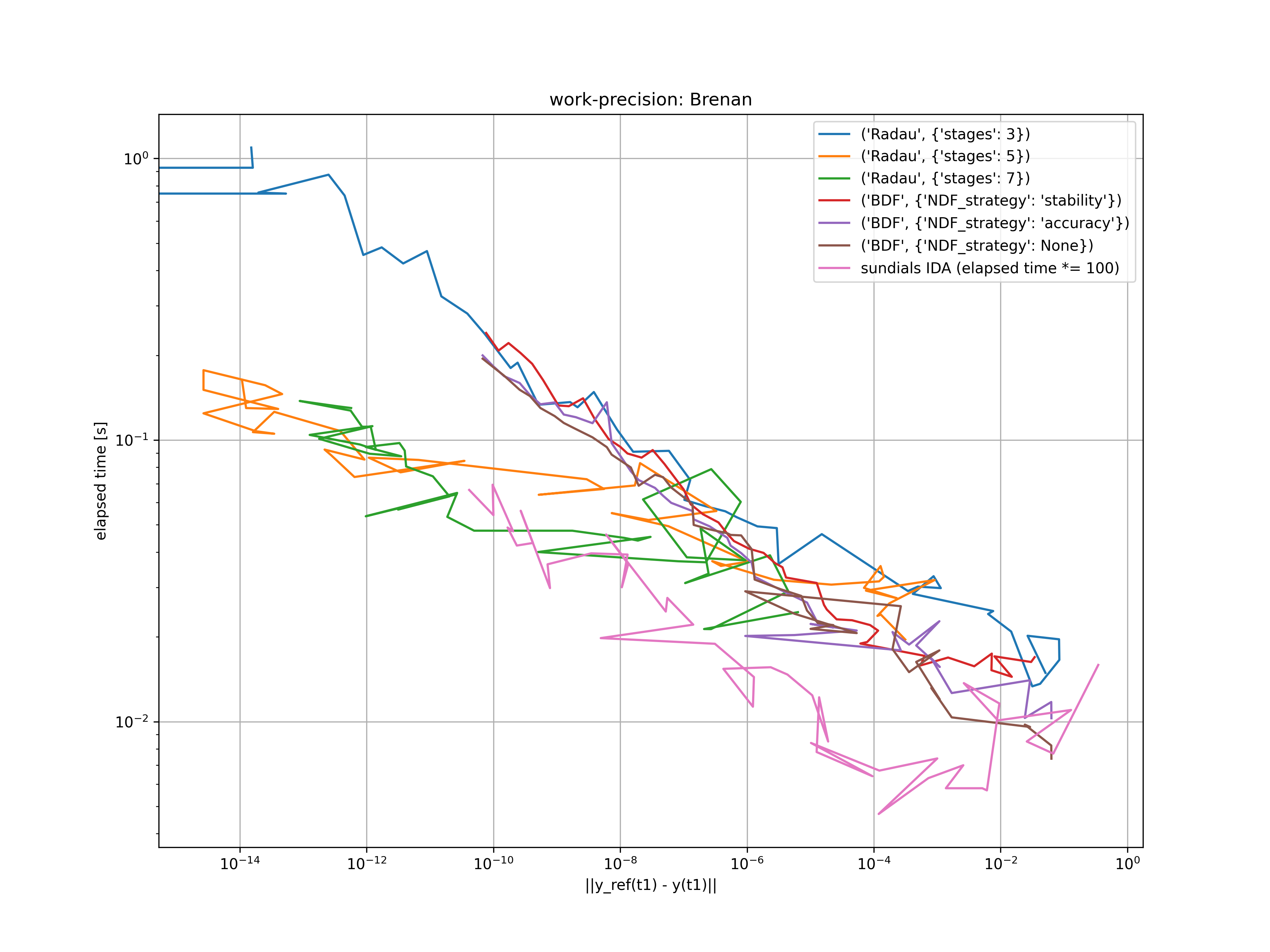
Clearly, the family of Radau IIA methods outplay the BDF/NDF methods for low tolerances. For medium to high tolerances, both methods are appropriate.
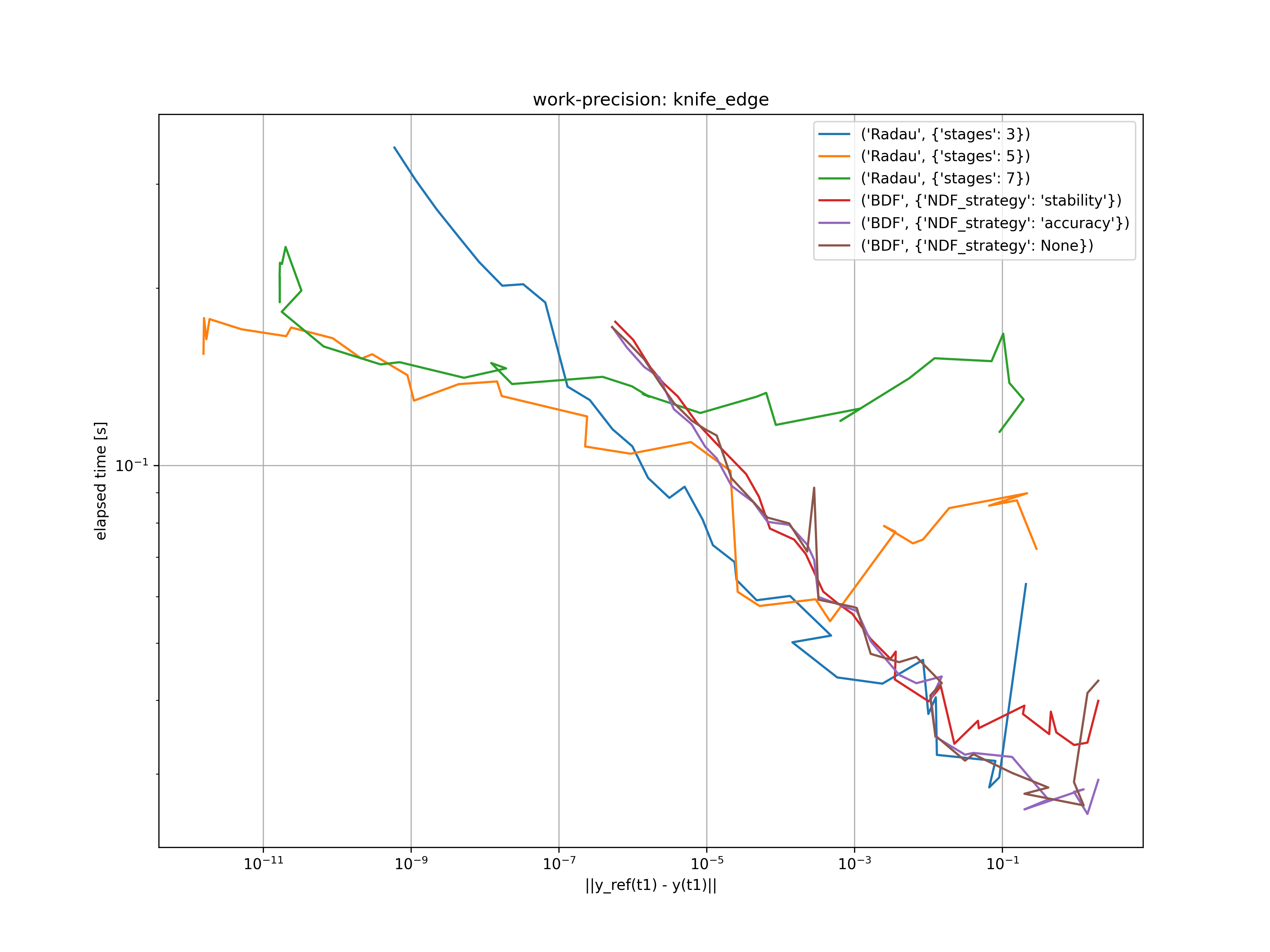
### Index 2 DAE - knife edge
The [knife edge index 2 problem](https://doi.org/10.1007/978-1-4939-3017-3) is a simple mechanical example with nonholonomic constraint. It is described by the system of differential algebraic equations
$$
\begin{aligned}
\dot{x} &= u \\
\dot{y} &= v \\
\dot{\varphi} &= \omega \\
m \dot{u} &= m g \sin\alpha + \sin\varphi \lambda \\
m \dot{v} &= -\cos\varphi \lambda \\
J \dot{\omega} &= 0 \\
0 &= u \sin\varphi - v \cos\varphi .
\end{aligned}
$$
Since the implemented solvers are designed for index 1 DAEs we have to perform some sort of index reduction. Therefore, we transform the semi-explicit form into a general form as proposed by [Gear](https://doi.org/10.1137/0909004). The resulting index 1 system is given as
$$
\begin{aligned}
\dot{x} &= u \\
\dot{y} &= v \\
\dot{\varphi} &= \omega \\
m \dot{u} &= m g \sin\alpha + \sin\varphi \dot{\Lambda} \\
m \dot{v} &= -\cos\varphi \dot{\Lambda} \\
J \dot{\omega} &= 0 \\
0 &= u \sin\varphi - v \cos\varphi .
\end{aligned}
$$
For the initial conditions $t_0 = 0$, $x(t_0) = \dot{x}(t_0) = y(t_0) = \dot{y}(t_0) = \varphi(t_0) = 0$ and $\dot{\varphi}(t_0) = \Omega$, a closed form solution is given by
$$
\begin{aligned}
x(t) &= \frac{g \sin\alpha}{2 \Omega^2} \sin^2(\Omega t) \\
y(t) &= \frac{g \sin\alpha}{2 \Omega^2} \left(\Omega t - \frac{1}{2}\sin(2 \Omega t)\right) \\
\varphi(t) &= \Omega t \\
u(t) &= \frac{g \sin\alpha}{\Omega} \sin(\Omega t) \cos(\Omega t) \\
v(t) &= \frac{g \sin\alpha}{2 \Omega} \left(1 - \cos(2 \Omega t)\right) = \frac{g \sin\alpha}{\Omega} \sin^2(\Omega t) \\
\omega(t) &= \Omega \\
\Lambda(t) &= \frac{2g \sin\alpha}{\Omega} (\cos(\Omega t) - 1) ,
% (2 * m * g * salpha / Omega) * (np.cos(Omega * t) - 1)
\end{aligned}
$$
with the Lagrange multiplier $\dot{\Lambda}(t) = - 2g \sin\alpha \sin(\Omega t)$.
This problem is solved for $atol = rtol = 10^{-(1 + m / 4)}$, where $m = 0, \dots, 32$. The resulting error at $t_1 = 2 \pi / \Omega$ is compared with the elapsed time of the used solvers in the figure below.
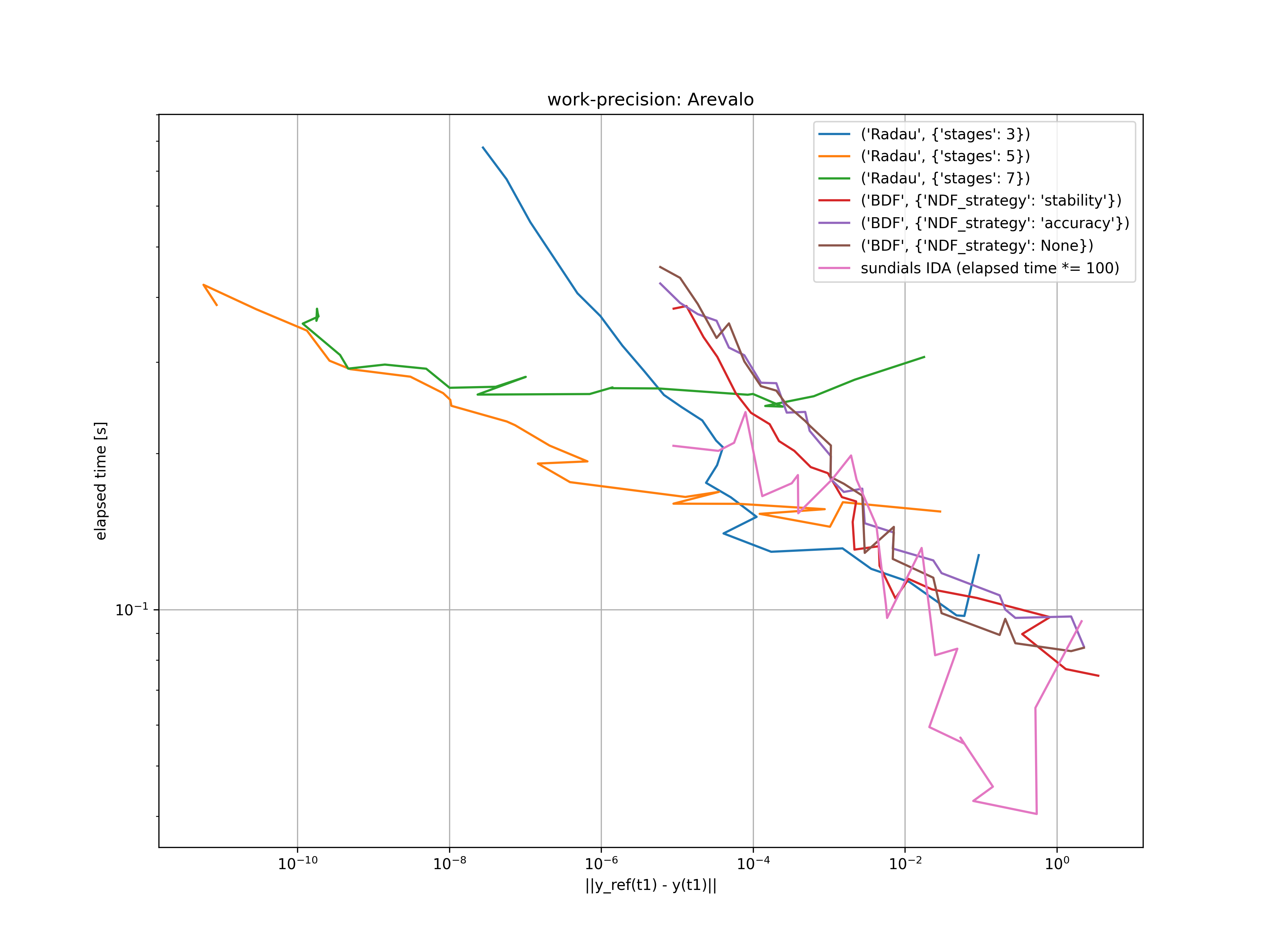
### Index 3 DAE - Arevalo
[Arevalo's index 3 problem](https://link.springer.com/article/10.1007/BF01732606) describes the motion of a particle on a circular track. It is described by the system of differential algebraic equations
$$
\begin{aligned}
\dot{x} &= u \\
\dot{y} &= v \\
\dot{u} &= 2 y + x \lambda \\
\dot{v} &= -2 x + y \lambda \\
0 &= x^2 + y^2 - 1 .
\end{aligned}
$$
Since the implemented solvers are designed for index 1 DAEs we have to perform some sort of index reduction. Therefore, we use the [stabilized index 1 formulation of Hiller and Anantharaman](https://doi.org/10.1002/nme.1620320803). The resulting index 1 system is given as
$$
\begin{aligned}
\dot{x} &= u + x \dot{\Gamma} \\
\dot{y} &= v + y \dot{\Gamma} \\
\dot{u} &= 2 y + x \dot{\Lambda} \\
\dot{v} &= -2 x + y \dot{\Lambda} \\
0 &= x u + y v \\
0 &= x^2 + y^2 - 1 .
\end{aligned}
$$
The analytical solution to this problem is given by
$$
\begin{aligned}
x(t) &= \sin(t^2) \\
y(t) &= \cos(t^2) \\
u(t) &= 2 t \cos(t^2) \\
v(t) &= -2 t \sin(t^2) \\
\Lambda(t) &= -\frac{4}{3} t^3 \\
\Gamma(t) &= 0 ,
\end{aligned}
$$
with the Lagrange multipliers $\dot{\Lambda} = -4t^2$ and $\dot{\Gamma} = 0$.
This problem is solved for $atol = rtol = 10^{-(3 + m / 4)}$, where $m = 0, \dots, 24$. The resulting error at $t_1 = 5$ is compared with the elapsed time of the used solvers in the figure below.
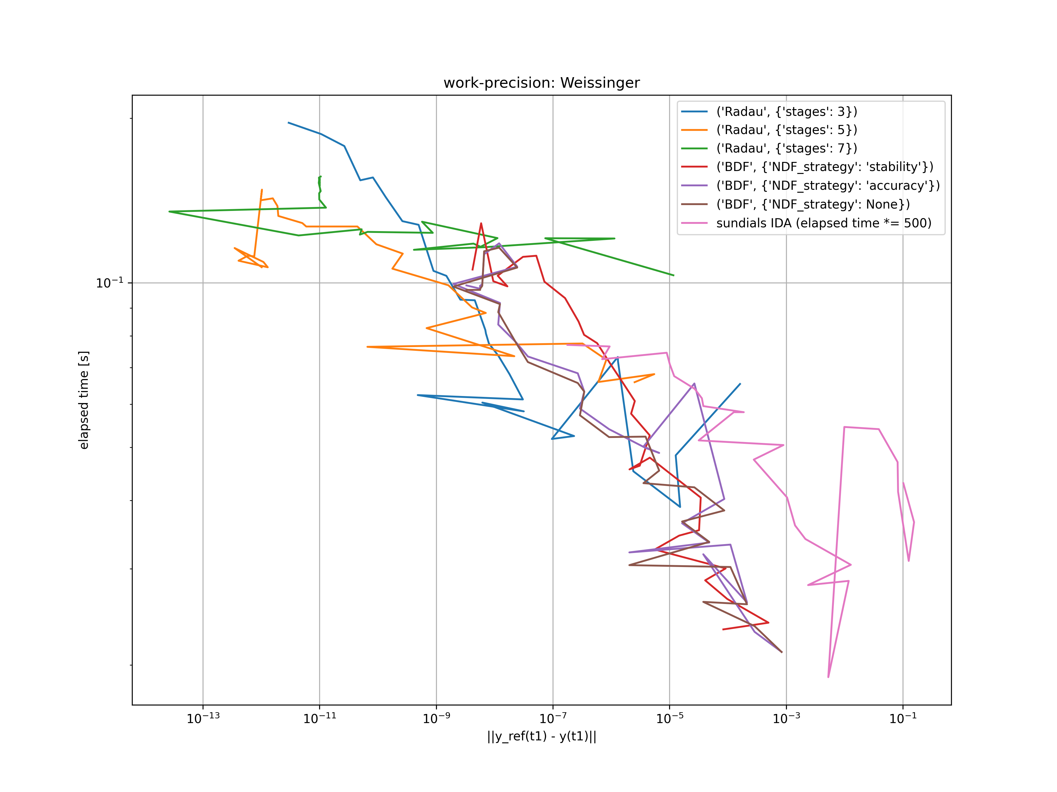
### IDE - Weissinger
A simple example of an implicit differential equations is called [Weissinger's equation](https://www.mathworks.com/help/matlab/ref/ode15i.html#bu7u4dt-1)
$$
t y^2 (\dot{y})^3 - y^3 (\dot{y}^2) + t (t^2 + 1) \dot{y} - t^2 y = 0 .
$$
It has the analytical solution $y(t) = \sqrt{t^2 + \frac{1}{2}}$ and $\dot{y}(t) = \frac{t}{\sqrt{t^2 + \frac{1}{2}}}$.
Starting at $t_0 = \sqrt{1 / 2}$, this problem is solved for $atol = rtol = 10^{-(4 + m / 4)}$, where $m = 0, \dots, 28$. The resulting error at $t_1 = 10$ is compared with the elapsed time of the used solvers in the figure below.
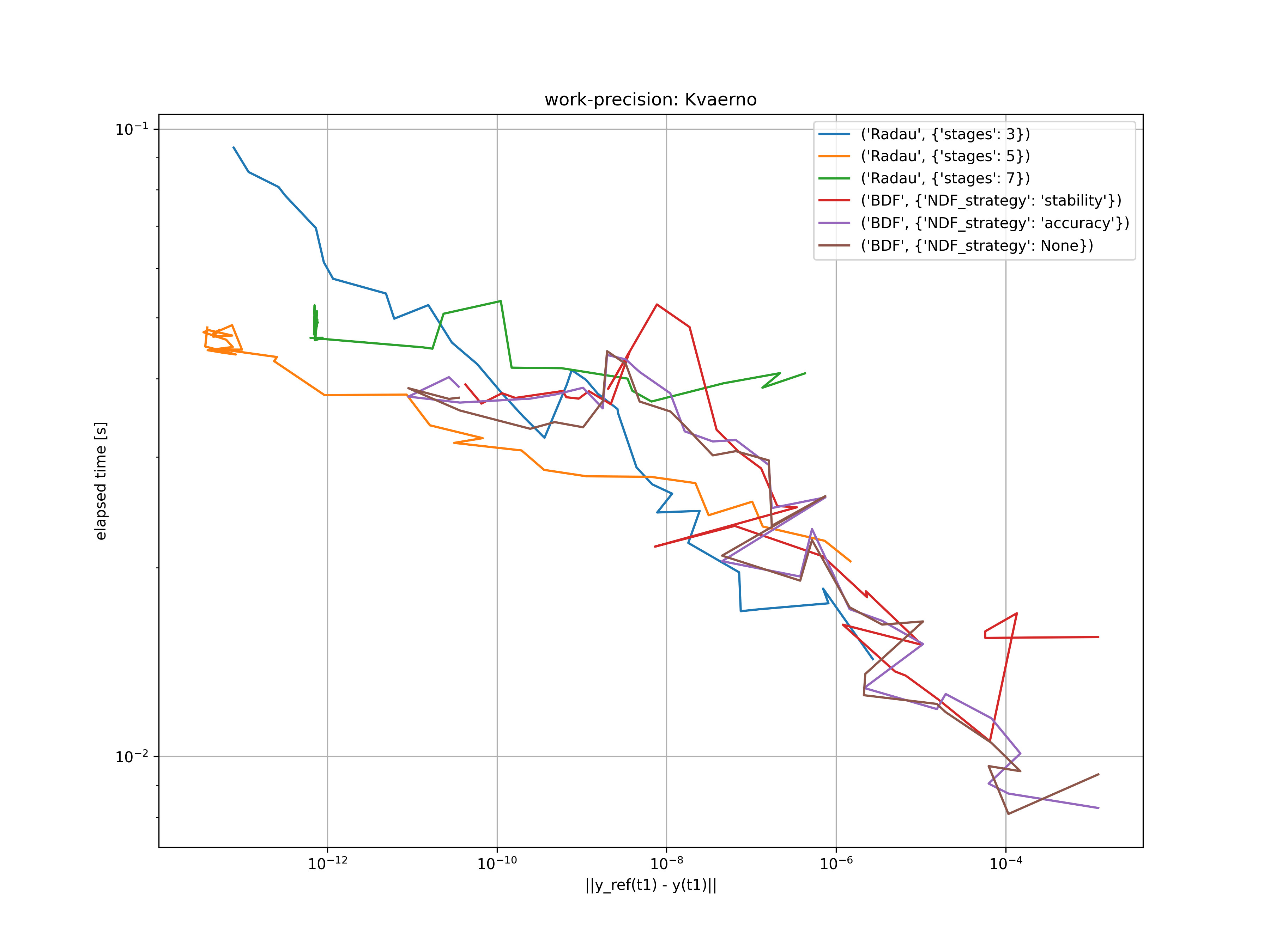
### Nonlinear index 1 DAE - Kvaernø
In a final example, an nonlinear index 1 DAE is investigated as proposed by [Kvaernø](https://doi.org/10.2307/2008502). The system is given by
$$
\begin{aligned}
(\sin^2(\dot{y}_1) + \sin^2(y_2)) (\dot{y}_2)^2 - (t - 6)^2 (t - 2)^2 y_1 e^{-t} &= 0 \\
(4 - t) (y_2 + y_1)^3 - 64 t^2 e^{-t} y_1 y_2 &= 0 ,
\end{aligned}
$$
It has the analytical solution $y_1(t) = t^4 e^{-t}$, $y_2(t) = t^3 e^{-t} (4 - t)$ and $\dot{y}_1(t) = (4 t^3 - t^4) e^{-t}$, $y_2(t) = (-t^3 + (4 - t) 3 t^2 - (4 - t) t^3) e^{-t}$.
Starting at $t_0 = 0.5$, this problem is solved for $atol = rtol = 10^{-(4 + m / 4)}$, where $m = 0, \dots, 32$. The resulting error at $t_1 = 1$ is compared with the elapsed time of the used solvers in the figure below.
## Install
### Install through pip
To install scipy-dae package you can run the command
```
pip install scipy-dae
```
### Install through git repository
To install the package through git installation you can download the repository and install it through
```
pip install .
```
### Install for developing and testing
An editable developer mode can be installed via
```bash
python -m pip install -e .[dev]
```
The tests can be started using
```bash
python -m pytest --cov
```