https://github.com/loliverhennigh/phy-net
compressing physics with neural networks
https://github.com/loliverhennigh/phy-net
cfd fluid-simulation mechsys neural-network simulation
Last synced: 11 months ago
JSON representation
compressing physics with neural networks
- Host: GitHub
- URL: https://github.com/loliverhennigh/phy-net
- Owner: loliverhennigh
- License: apache-2.0
- Created: 2016-11-05T16:12:09.000Z (over 9 years ago)
- Default Branch: master
- Last Pushed: 2018-07-10T16:33:25.000Z (almost 8 years ago)
- Last Synced: 2024-11-21T17:05:44.835Z (over 1 year ago)
- Topics: cfd, fluid-simulation, mechsys, neural-network, simulation
- Language: Python
- Size: 175 MB
- Stars: 152
- Watchers: 19
- Forks: 55
- Open Issues: 0
-
Metadata Files:
- Readme: README.md
- License: License.md
Awesome Lists containing this project
README
# Lat-Net: Compressing Lattice Boltzmann Flow Simulations using Deep Neural Networks
## Introduction
This repository contains the code to reproduce results seen in [Lat-Net: Compressing Lattice Boltzmann Flow Simulations using Deep Neural Networks](https://arxiv.org/abs/1705.09036). The premise is to compress Lattice Boltzmann Fluid Flow simulations onto small computationally efficient neural networks that can be evaluated.
## Related Work
Similar works can be found in "[Accelerating Eulerian Fluid Simulation With Convolutional Networks](https://arxiv.org/pdf/1607.03597.pdf)" and "[Convolutional Neural Networks for steady Flow Approximation](https://autodeskresearch.com/publications/convolutional-neural-networks-steady-flow-approximation)".
## Network Details

The network learns a encoding, compression, and decoding piece. The encoding piece learns to compress the state of the physics simulation. The compression piece learns the dynamics of the simulation on this compressed piece. The decoding piece learns to decode the compressed representation. The network is kept all convolutional allowing it to be trained and evaluated on any size simulation. This means that once the model is trained on a small simulation (say 256 by 256 grid) it can then attempt to simulate the dynamics of a larger simulation (say 1024 by 1024 grid). We show that the model can still produce accurate results even with larger simulations then seen during training.
## Lattice Boltzmann Fluid Flow
Using the Mechsys library we generated 2D and 3D fluid simulations to train our model. For the 2D case we simulate a variety of random objects interacting with a steady flow and periodic boundary conditions. The simulation is a 256 by 256 grid. Using the trained model we evaluate on grid size 256 by 256, 512 by 512, and 1024 by 1024. Here are examples of generated simulations.
[](https://www.youtube.com/watch?v=Nuf_Jw4fGFk)
[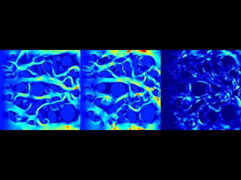](https://www.youtube.com/watch?v=YtsQX9L56Dg)
[](https://www.youtube.com/watch?v=vPrHXMlDW0k)
We can look at various properties of the true versus generated simulations such as mean squared error, divergence of the velocity vector field, drag, and flux. Averaging over several test simulations we see the that the generated simulation produces realistic values. The following graphs show this for 256, 512, and 1024 sized simulations.


A few more snap shots of simulations


Now we can apply it to other datasets. Here is a simulation around a car cross section. This demonstrates that our method generalizes to vastly different geometries.

[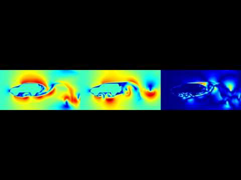](https://www.youtube.com/watch?v=bX0_4zjYtHo)
Here are some 3D simulations.
[](https://www.youtube.com/watch?v=ZG_gmkFbE2I)
[](https://www.youtube.com/watch?v=ilCuHTo0Ul4)
Here are the plots for the 3D simulations.


## Lattice Boltzmann Electromagnetic Waves
Well the Lattice Boltzmann method is actually a general partial differential equation solver (of a particular form) so why stop at fluid flow! Here are some fun electromagnetic simulations that the model learns. These simulations are of a wave hitting randomly placed objects with different dielectric constants. You can see fun effects such as reflection and refraction when the wave interacts with the surface.
[](https://www.youtube.com/watch?v=s57No66p_40)
[](https://www.youtube.com/watch?v=jaYd1YLDzXo)
Here are the plots for EM simulations


## How to run
Running the 2d simulations requires around 100 Gb of hard drive memory, a good gpu (currently using GTX 1080s), and 1 and a half days. The 3d simulations can take substantially longer.
### Generating Data
The test and train sets are generated using the [Mechsys library](http://mechsys.nongnu.org/index.html). Follow the installation guild found [here](http://mechsys.nongnu.org/installation.html). Once the directory is unpacked run `ccmake .` followed by `c`. Then scroll to the flag that says `A_USE_OCL` and hit enter to raise the flag. Press `c` again to configure followed by `g` to generate (I found ccmake to be confusing at first). Quit the prompt and run `make`. Now copy the contents of `Phy-Net/systems/mechsys_fluid_flow` to the directory `mechsys/tflbm` as well as replace `mechsys/lib/flbm/Domain.h` with the one found in this directory. Now enter `mechsys/tflbm` and run `make` followed by
`
./generate_data
`.
This will generate the required train and test set for the 2D simulations and save them to `/data/` (this can be changed in the `run_bunch_2d` script. 3D simulation is commented out for now. Generating the 2D simulation data will require about 12 hours.
Generating the data to train on is by far the most complicated piece of this work. It requires several external packages and considerable memory. I recently wrote a library to generate Lattice Boltzmann simulations entirely in Tensorflow [here](https://github.com/loliverhennigh/Lattice-Boltzmann-fluid-flow-in-Tensorflow). In the future I would like to integrate this library with the train code allowing the data generation to be streamlined.
### Train Model
To train the model enter the `Phy-Net/train` directory and run
`
python compress_train.py
`
This will first generate tfrecords for the generated training data and then begin training. Multi GPU training is supported with the flag `--nr_gpu=n` for `n` gpus. The important flags for training and model configurations are
- `--nr_residual=2` Number of residual blocks in each downsample chunk of the encoder and decoder
- `--nr_downsamples=4` Number of downsamples in the encoder and decoder
- `--filter_size=8` Number of filters for the first encoder layer. The filters double after each downsample.
- `--nr_residual_compression=3` Number of residual blocks in compression piece.
- `--filter_size_compression=64` filter size of residual blocks in compression piece.
- `--unroll_length=5` Number of steps in the future the network is unrolled.
All flags and their uses can be found in `Phy-Net/model/ring_net.py`.
### Test Model
There are several different tests that can be run in the test directory. For the 2D simulations, running these scripts will generate the figures and videos above.
- `2d_error_test.txt` Generates the error plots seen above
- `2d_image_test.txt` Generates the images seen above
- `2d_video_test.txt` Generates the videos seen above
### Contact
For any questions regarding the project please email me at loliverhennigh101@gmail.com.