https://github.com/lsys/forestplot
A Python package to make publication-ready but customizable coefficient plots.
https://github.com/lsys/forestplot
coefficientplot data-science data-visualization dataviz forestplot matplotlib python visualization
Last synced: about 1 year ago
JSON representation
A Python package to make publication-ready but customizable coefficient plots.
- Host: GitHub
- URL: https://github.com/lsys/forestplot
- Owner: LSYS
- License: mit
- Created: 2022-07-03T12:11:42.000Z (almost 4 years ago)
- Default Branch: main
- Last Pushed: 2024-07-28T07:20:29.000Z (almost 2 years ago)
- Last Synced: 2024-10-06T02:07:44.816Z (over 1 year ago)
- Topics: coefficientplot, data-science, data-visualization, dataviz, forestplot, matplotlib, python, visualization
- Language: Jupyter Notebook
- Homepage: http://forestplot.rtfd.io
- Size: 8.38 MB
- Stars: 111
- Watchers: 3
- Forks: 10
- Open Issues: 6
-
Metadata Files:
- Readme: README.md
- License: LICENSE
- Citation: citation.cff
Awesome Lists containing this project
README
Forestplot

Easy API for forest plots.
A Python package to make publication-ready but customizable forest plots.
-----------------------------------------------------------
This package makes publication-ready forest plots easy to make out-of-the-box. Users provide a `dataframe` (e.g. from a spreadsheet) where rows correspond to a variable/study with columns including estimates, variable labels, and lower and upper confidence interval limits.
Additional options allow easy addition of columns in the `dataframe` as annotations in the plot.
| | |
| --- | --- |
| Release | [](https://pypi.org/project/forestplot/) [](https://anaconda.org/conda-forge/forestplot) [](https://github.com/LSYS/forestplot/releases) |
| Status | [](https://github.com/LSYS/forestplot/actions/workflows/CI.yml) [](https://github.com/LSYS/forestplot/actions/workflows/nb.yml) |
| Coverage | [](https://app.codecov.io/gh/LSYS/forestplot) |
| Python | [](https://pypi.org/project/forestplot/) |
| Docs | [](https://forestplot.readthedocs.io/en/latest/?badge=latest) [](https://github.com/LSYS/forestplot/actions/workflows/links.yml)|
| Meta | [](https://choosealicense.com/licenses/mit/) [](https://pycqa.github.io/isort/) [](https://github.com/psf/black) [](https://github.com/python/mypy) [](https://zenodo.org/badge/latestdoi/510013191) |
| Binder| [](https://mybinder.org/v2/gh/lsys/forestplot/main?labpath=examples%2Freadme-examples.ipynb) |
# Table of Contents[](#table-of-contents)
show/hide
> - [Installation](#installation)
> - [Quick Start](#quick-start)
> - [Some Examples with Customizations](#some-examples-with-customizations)
> - [Gallery and API Options](#gallery-and-api-options)
> - [Multi-models](#multi-models)
> - [Known Issues](#known-issues)
> - [Background and Additional Resources](#background-and-additional-resources)
> - [Contributing](#contributing)
## Installation[](#installation)
Install from PyPI
[](https://pypi.org/project/forestplot/)
```bash
pip install forestplot
```
Install from conda-forge
[](https://anaconda.org/conda-forge/forestplot)
```bash
conda install forestplot
```
Install from source
[](https://github.com/LSYS/forestplot/releases)
```bash
git clone https://github.com/LSYS/forestplot.git
cd forestplot
pip install .
```
Developer installation
```bash
git clone https://github.com/LSYS/forestplot.git
cd forestplot
pip install -r requirements_dev.txt
make lint
make test
```
## Quick Start[](#quick-start)
```python
import forestplot as fp
df = fp.load_data("sleep") # companion example data
df.head(3)
```
| | var | r | moerror | label | group | ll | hl | n | power | p-val |
|---:|:---------|-----------:|----------:|:--------------------------|:--------------|------:|------:|----:|---------:|----------:|
| 0 | age | 0.0903729 | 0.0696271 | in years | age | 0.02 | 0.16 | 706 | 0.671578 | 0.0163089 |
| 1 | black | -0.0270573 | 0.0770573 | =1 if black | other factors | -0.1 | 0.05 | 706 | 0.110805 | 0.472889 |
| 2 | clerical | 0.0480811 | 0.0719189 | =1 if clerical worker | occupation | -0.03 | 0.12 | 706 | 0.247768 | 0.201948 |
(* This is a toy example of how certain factors correlate with the amount of sleep one gets. See the [notebook that generates the data](https://nbviewer.org/github/LSYS/forestplot/blob/main/examples/get-sleep.ipynb).)
The example input dataframe above have 4 key columns
| Column | Description | Required |
|:----------|:------------------------------------------------|:----------|
| `var` | Variable label | ✓ |
| `r` | Correlation coefficients (estimates to plot) | ✓ |
| `label` | Variable labels | ✓ |
| `group` | Variable grouping labels | |
| `ll` | Conf. int. *lower limits* | |
| `hl` | Containing the conf. int. *higher limits* | |
| `n` | Sample size | |
| `power` | Statistical power | |
| `p-val` | P-value | |
(See [Gallery and API Options](#gallery-and-api-options) for more details on required and optional arguments.)
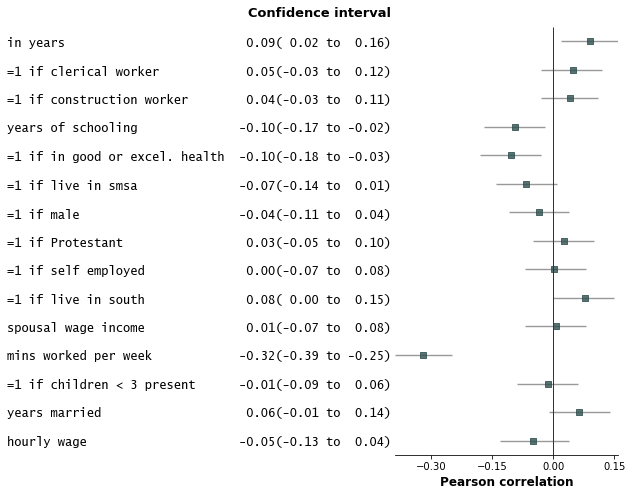
Make the forest plot
```python
fp.forestplot(df, # the dataframe with results data
estimate="r", # col containing estimated effect size
ll="ll", hl="hl", # columns containing conf. int. lower and higher limits
varlabel="label", # column containing variable label
ylabel="Confidence interval", # y-label title
xlabel="Pearson correlation", # x-label title
)
```
Save the plot
```python
plt.savefig("plot.png", bbox_inches="tight")
```
## Some Examples With Customizations[](#some-examples-with-customizations)
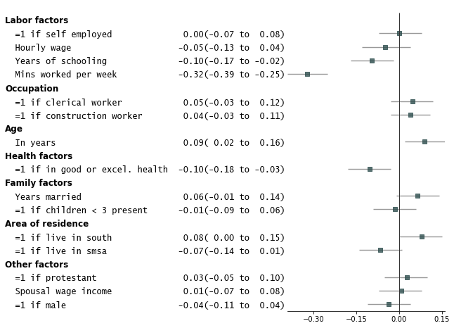
1. Add variable groupings, add group order, and sort by estimate size.
```python
fp.forestplot(df, # the dataframe with results data
estimate="r", # col containing estimated effect size
ll="ll", hl="hl", # columns containing conf. int. lower and higher limits
varlabel="label", # column containing variable label
capitalize="capitalize", # Capitalize labels
groupvar="group", # Add variable groupings
# group ordering
group_order=["labor factors", "occupation", "age", "health factors",
"family factors", "area of residence", "other factors"],
sort=True # sort in ascending order (sorts within group if group is specified)
)
```
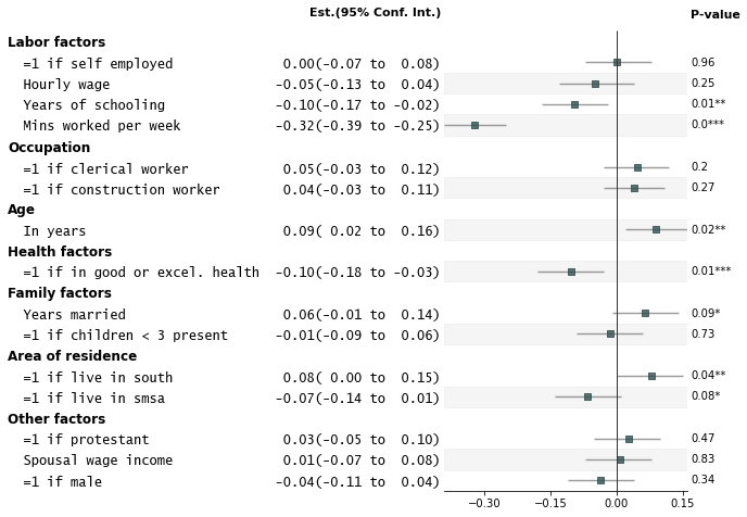
2. Add p-values on the right and color alternate rows gray
```python
fp.forestplot(df, # the dataframe with results data
estimate="r", # col containing estimated effect size
ll="ll", hl="hl", # columns containing conf. int. lower and higher limits
varlabel="label", # column containing variable label
capitalize="capitalize", # Capitalize labels
groupvar="group", # Add variable groupings
# group ordering
group_order=["labor factors", "occupation", "age", "health factors",
"family factors", "area of residence", "other factors"],
sort=True, # sort in ascending order (sorts within group if group is specified)
pval="p-val", # Column of p-value to be reported on right
color_alt_rows=True, # Gray alternate rows
ylabel="Est.(95% Conf. Int.)", # ylabel to print
**{"ylabel1_size": 11} # control size of printed ylabel
)
```
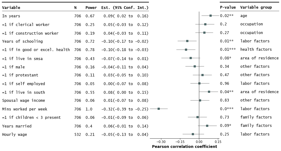
3. Customize annotations and make it a table
```python
fp.forestplot(df, # the dataframe with results data
estimate="r", # col containing estimated effect size
ll="ll", hl="hl", # lower & higher limits of conf. int.
varlabel="label", # column containing the varlabels to be printed on far left
capitalize="capitalize", # Capitalize labels
pval="p-val", # column containing p-values to be formatted
annote=["n", "power", "est_ci"], # columns to report on left of plot
annoteheaders=["N", "Power", "Est. (95% Conf. Int.)"], # ^corresponding headers
rightannote=["formatted_pval", "group"], # columns to report on right of plot
right_annoteheaders=["P-value", "Variable group"], # ^corresponding headers
xlabel="Pearson correlation coefficient", # x-label title
table=True, # Format as a table
)
```
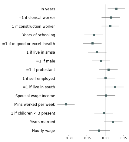
4. Strip down all bells and whistle
```python
fp.forestplot(df, # the dataframe with results data
estimate="r", # col containing estimated effect size
ll="ll", hl="hl", # lower & higher limits of conf. int.
varlabel="label", # column containing the varlabels to be printed on far left
capitalize="capitalize", # Capitalize labels
ci_report=False, # Turn off conf. int. reporting
flush=False, # Turn off left-flush of text
**{'fontfamily': 'sans-serif'} # revert to sans-serif
)
```
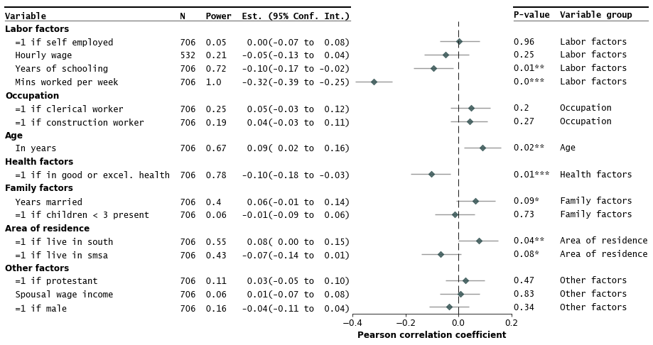
5. Example with more customizations
```python
fp.forestplot(df, # the dataframe with results data
estimate="r", # col containing estimated effect size
ll="ll", hl="hl", # lower & higher limits of conf. int.
varlabel="label", # column containing the varlabels to be printed on far left
capitalize="capitalize", # Capitalize labels
pval="p-val", # column containing p-values to be formatted
annote=["n", "power", "est_ci"], # columns to report on left of plot
annoteheaders=["N", "Power", "Est. (95% Conf. Int.)"], # ^corresponding headers
rightannote=["formatted_pval", "group"], # columns to report on right of plot
right_annoteheaders=["P-value", "Variable group"], # ^corresponding headers
groupvar="group", # column containing group labels
group_order=["labor factors", "occupation", "age", "health factors",
"family factors", "area of residence", "other factors"],
xlabel="Pearson correlation coefficient", # x-label title
xticks=[-.4,-.2,0, .2], # x-ticks to be printed
sort=True, # sort estimates in ascending order
table=True, # Format as a table
# Additional kwargs for customizations
**{"marker": "D", # set maker symbol as diamond
"markersize": 35, # adjust marker size
"xlinestyle": (0, (10, 5)), # long dash for x-reference line
"xlinecolor": "#808080", # gray color for x-reference line
"xtick_size": 12, # adjust x-ticker fontsize
}
)
```

Annotations arguments allowed include:
* `ci_range`: Confidence interval range (e.g. `(-0.39 to -0.25)`).
* `est_ci`: Estimate and CI (e.g. `-0.32(-0.39 to -0.25)`).
* `formatted_pval`: Formatted p-values (e.g. `0.01**`).
To confirm what processed `columns` are available as annotations, you can do:
```python
processed_df, ax = fp.forestplot(df,
... # other arguments here
return_df=True # return processed dataframe with processed columns
)
processed_df.head(3)
```
| | label | group | n | r | CI95% | p-val | BF10 | power | var | hl | ll | moerror | formatted_r | formatted_ll | formatted_hl | ci_range | est_ci | formatted_pval | formatted_n | formatted_power | formatted_est_ci | yticklabel | formatted_formatted_pval | formatted_group | yticklabel2 |
|---:|:---------------------|:--------------|----:|-----------:|:--------------|------------:|----------:|--------:|:-------|------:|------:|----------:|--------------:|---------------:|---------------:|:-----------------|:----------------------|:-----------------|--------------:|------------------:|:----------------------|:------------------------------------------------------------------|:---------------------------|:------------------|:-----------------------|
| 0 | Mins worked per week | Labor factors | 706 | -0.321384 | [-0.39 -0.25] | 1.99409e-18 | 1.961e+15 | 1 | totwrk | -0.25 | -0.39 | 0.0686165 | -0.32 | -0.39 | -0.25 | (-0.39 to -0.25) | -0.32(-0.39 to -0.25) | 0.0*** | 706 | 1 | -0.32(-0.39 to -0.25) | Mins worked per week 706 1.0 -0.32(-0.39 to -0.25) | 0.0*** | Labor factors | 0.0*** Labor factors |
| 1 | Years of schooling | Labor factors | 706 | -0.0950039 | [-0.17 -0.02] | 0.0115515 | 1.137 | 0.72 | educ | -0.02 | -0.17 | 0.0749961 | -0.1 | -0.17 | -0.02 | (-0.17 to -0.02) | -0.10(-0.17 to -0.02) | 0.01** | 706 | 0.72 | -0.10(-0.17 to -0.02) | Years of schooling 706 0.72 -0.10(-0.17 to -0.02) | 0.01** | Labor factors | 0.01** Labor factors |
## Multi-models[](#multi-models)
For coefficient plots where each variable can have multiple estimates (each `model` has one).
```python
import forestplot as fp
df_mmodel = pd.read_csv("../examples/data/sleep-mmodel.csv").query(
"model=='all' | model=='young kids'"
)
df_mmodel.head(3)
```
| | var | coef | se | T | pval | r2 | adj_r2 | ll | hl | model | group | label |
|---:|:------|-----------:|---------:|----------:|---------:|---------:|-----------:|-----------:|--------:|:-----------|:--------------|:------------|
| 0 | age | 0.994889 | 1.96925 | 0.505213 | 0.613625 | 0.127289 | 0.103656 | -2.87382 | 4.8636 | all | age | in years |
| 3 | age | 22.634 | 15.4953 | 1.4607 | 0.149315 | 0.178147 | -0.0136188 | -8.36124 | 53.6293 | young kids | age | in years |
| 4 | black | -84.7966 | 82.1501 | -1.03222 | 0.302454 | 0.127289 | 0.103656 | -246.186 | 76.5925 | all | other factors | =1 if black |
```python
fp.mforestplot(
dataframe=df_mmodel,
estimate="coef",
ll="ll",
hl="hl",
varlabel="label",
capitalize="capitalize",
model_col="model",
color_alt_rows=True,
groupvar="group",
table=True,
rightannote=["var", "group"],
right_annoteheaders=["Source", "Group"],
xlabel="Coefficient (95% CI)",
modellabels=["Have young kids", "Full sample"],
xticks=[-1200, -600, 0, 600],
mcolor=["#CC6677", "#4477AA"],
# Additional kwargs for customizations
**{
"markersize": 30,
# override default vertical offset between models (0.0 to 1.0)
"offset": 0.35,
"xlinestyle": (0, (10, 5)), # long dash for x-reference line
"xlinecolor": ".8", # gray color for x-reference line
},
)
```
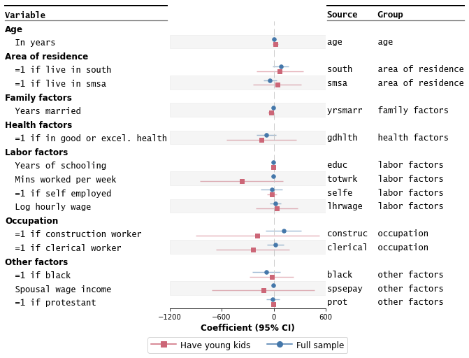
Please note: This module is still experimental. See [this jupyter notebook](https://nbviewer.org/github/LSYS/forestplot/blob/mplot-dev/examples/test-multmodel-sleep.ipynb) for more examples and tweaks.
## Gallery and API Options[](#gallery-and-api-options)
[](https://github.com/LSYS/forestplot/actions/workflows/nb.yml)
Check out [this jupyter notebook](https://nbviewer.org/github/LSYS/forestplot/blob/main/examples/readme-examples.ipynb) for a gallery variations of forest plots possible out-of-the-box.
The table below shows the list of arguments users can pass in.
More fined-grained control for base plot options (eg font sizes, marker colors) can be inferred from the [example notebook gallery](https://nbviewer.org/github/LSYS/forestplot/blob/main/examples/readme-examples.ipynb).
| Option | Description | Required |
|:-------------|:-------------------------------------------------------------------------------------------------------------------------------------------------------------|:---|
| `dataframe` | Pandas dataframe where rows are variables (or studies for meta-analyses) and columns include estimated effect sizes, labels, and confidence intervals, etc. | ✓ |
| `estimate` | Name of column in `dataframe` containing the *estimates*. | ✓ |
| `varlabel` | Name of column in `dataframe` containing the *variable labels* (study labels if meta-analyses). | ✓ |
| `ll` | Name of column in `dataframe` containing the conf. int. *lower limits*. | |
| `hl` | Name of column in `dataframe` containing the conf. int. *higher limits*. | |
| `logscale` | If True, make the x-axis log scale. Default is False. | |
| `capitalize` | How to capitalize strings. Default is None. One of "capitalize", "title", "lower", "upper", "swapcase". | |
| `form_ci_report` | If True (default), report the estimates and confidence interval beside the variable labels. | |
| `ci_report` | If True (default), format the confidence interval as a string. | |
| `groupvar` | Name of column in `dataframe` containing the variable *grouping labels*. | |
| `group_order` | List of group labels indicating the order of groups to report in the plot. | |
| `annote` | List of columns to add as annotations on the left-hand side of the plot. | |
| `annoteheaders` | List of column headers for the left-hand side annotations. | |
| `rightannote` | List of columns to add as annotations on the right-hand side of the plot. | |
| `right_annoteheaders` | List of column headers for the right-hand side annotations. | |
| `pval` | Name of column in `dataframe` containing the p-values. | |
| `starpval` | If True (default), format p-values with stars indicating statistical significance. | |
| `sort` | If True, sort variables by `estimate` values in ascending order. | |
| `sortby` | Name of column to sort by. Default is `estimate`. | |
| `flush` | If True (default), left-flush variable labels and annotations. | |
| `decimal_precision` | Number of decimal places to print. (Default = 2) | |
| `figsize` | Tuple indicating core figure size. Default is (4, 8) | |
| `xticks` | List of xticklabels to print on x-axis. | |
| `ylabel` | Y-label title. | |
| `xlabel` | X-label title. | |
| `color_alt_rows` | If True, shade out alternating rows in gray. | |
| `preprocess` | If True (default), preprocess the `dataframe` before plotting. | |
| `return_df` | If True, returned the preprocessed `dataframe`. | |
## Known Issues[](#known-issues)
* Variable labels coinciding with group variables may lead to unexpected formatting issues in the graph.
* Left-flushing of annotations relies on the `monospace` font.
* Plot may give strange behavior for few rows of data (six rows or fewer. [see this issue](https://github.com/LSYS/forestplot/issues/52))
* Plot can get cluttered with too many variables/rows (~30 onwards)
* Not tested with PyCharm (#80) nor Google Colab (#110).
* Duplicated `varlabel` may lead to unexpected results (see #76, #81). `mplot` for grouped models could be useful for such cases (see #59, WIP).
## Background and Additional Resources[](#background-and-additional-resources)
**More about forest plots**
[Forest plots](https://en.wikipedia.org/wiki/Forest_plot) have many aliases (h/t Chris Alexiuk). Other names include coefplots, coefficient plots, meta-analysis plots, dot-and-whisker plots, blobbograms, margins plots, regression plots, and ropeladder plots.
[Forest plots](https://en.wikipedia.org/wiki/Forest_plot) in the medical and health sciences literature are plots that report results from different studies as a meta-analysis. Markers are centered on the estimated effect and horizontal lines running through each marker depicts the confidence intervals.
The simplest version of a forest plot has two columns: one for the variables/studies, and the second for the estimated coefficients and confidence intervals.
This layout is similar to coefficient plots ([coefplots](http://repec.sowi.unibe.ch/stata/coefplot/getting-started.html)) and is thus useful for more than meta-analyses.
More resources about forest plots
* [[1]](https://doi.org/10.1038/s41433-021-01867-6) Chang, Y., Phillips, M.R., Guymer, R.H. et al. The 5 min meta-analysis: understanding how to read and interpret a forest plot. Eye 36, 673–675 (2022).
* [[2]](https://doi.org/10.1136/bmj.322.7300.1479) Lewis S, Clarke M. Forest plots: trying to see the wood and the trees BMJ 2001; 322 :1479
**More about this package**
The package is lightweight, built on `pandas`, `numpy`, and `matplotlib`.
It is slightly opinioniated in that the aesthetics of the plot inherits some of my sensibilities about what makes a nice figure.
You can however easily override most defaults for the look of the graph. This is possible via `**kwargs` in the `forestplot` API (see [Gallery and API options](#gallery-and-api-options)) and the `matplotlib` API.
**Planned enhancements** include forest plots where each row can have multiple coefficients (e.g. from multiple models).
Related packages
* [[1]](https://www.stata-journal.com/article.html?article=gr0059) [Stata] Jann, Ben (2014). Plotting regression coefficients and other estimates. The Stata Journal 14(4): 708-737.
* [[2]](https://www.statsmodels.org/devel/examples/notebooks/generated/metaanalysis1.html) [Python] Meta-Analysis in statsmodels
* [[3]](https://github.com/seafloor/forestplot) [Python] Matt Bracher-Smith's Forestplot
* [[4]](https://github.com/fsolt/dotwhisker) [R] Solt, Frederick and Hu, Yue (2021) dotwhisker: Dot-and-Whisker Plots of Regression Results
* [[5]](https://rpubs.com/mbounthavong/forest_plots_r) [R] Bounthavong, Mark (2021) Forest plots. RPubs by RStudio
## Contributing[](#contributing)
Contributions are welcome, and they are greatly appreciated!
**Potential ways to contribute:**
* Raise issues/bugs/questions
* Write tests for missing coverage
* Add features (see [examples notebook](https://nbviewer.org/github/LSYS/forestplot/blob/main/examples/readme-examples.ipynb) for a survey of existing features)
* Add example datasets with companion graphs
* Add your graphs with companion code
**Issues**
Please submit bugs, questions, or issues you encounter to the [GitHub Issue Tracker](https://github.com/lsys/forestplot/issues).
For bugs, please provide a minimal reproducible example demonstrating the problem (it may help me troubleshoot if I have a version of your data).
**Pull Requests**
Please feel free to open an issue on the [Issue Tracker](https://github.com/lsys/forestplot/issues) if you'd like to discuss potential contributions via PRs.