https://github.com/matthiasnwt/fast-poisson-solver
The Poisson equation is an integral part of many physical phenomena, yet its computation is often time-consuming. This module presents an efficient method using physics-informed neural networks (PINNs) to rapidly solve arbitrary 2D Poisson problems.
https://github.com/matthiasnwt/fast-poisson-solver
math physics physics-2d physics-engine physics-informed-neural-networks physics-simulation pinn poisson poisson-equation poisson-equation-solver
Last synced: 3 months ago
JSON representation
The Poisson equation is an integral part of many physical phenomena, yet its computation is often time-consuming. This module presents an efficient method using physics-informed neural networks (PINNs) to rapidly solve arbitrary 2D Poisson problems.
- Host: GitHub
- URL: https://github.com/matthiasnwt/fast-poisson-solver
- Owner: matthiasnwt
- License: gpl-3.0
- Created: 2023-05-11T18:02:11.000Z (about 3 years ago)
- Default Branch: main
- Last Pushed: 2023-06-27T12:04:19.000Z (almost 3 years ago)
- Last Synced: 2025-12-15T12:45:15.880Z (6 months ago)
- Topics: math, physics, physics-2d, physics-engine, physics-informed-neural-networks, physics-simulation, pinn, poisson, poisson-equation, poisson-equation-solver
- Language: Python
- Homepage:
- Size: 20.4 MB
- Stars: 28
- Watchers: 1
- Forks: 1
- Open Issues: 2
-
Metadata Files:
- Readme: README.md
- Contributing: CONTRIBUTING.md
- License: LICENSE
- Code of conduct: CODE_OF_CONDUCT.md
Awesome Lists containing this project
README
# Fast Poisson Solver
The Poisson equation is an integral part of many physical phenomena, yet its computation
is often time-consuming. This module presents an efficient method using
physics-informed neural networks (PINNs) to rapidly solve arbitrary 2D Poisson
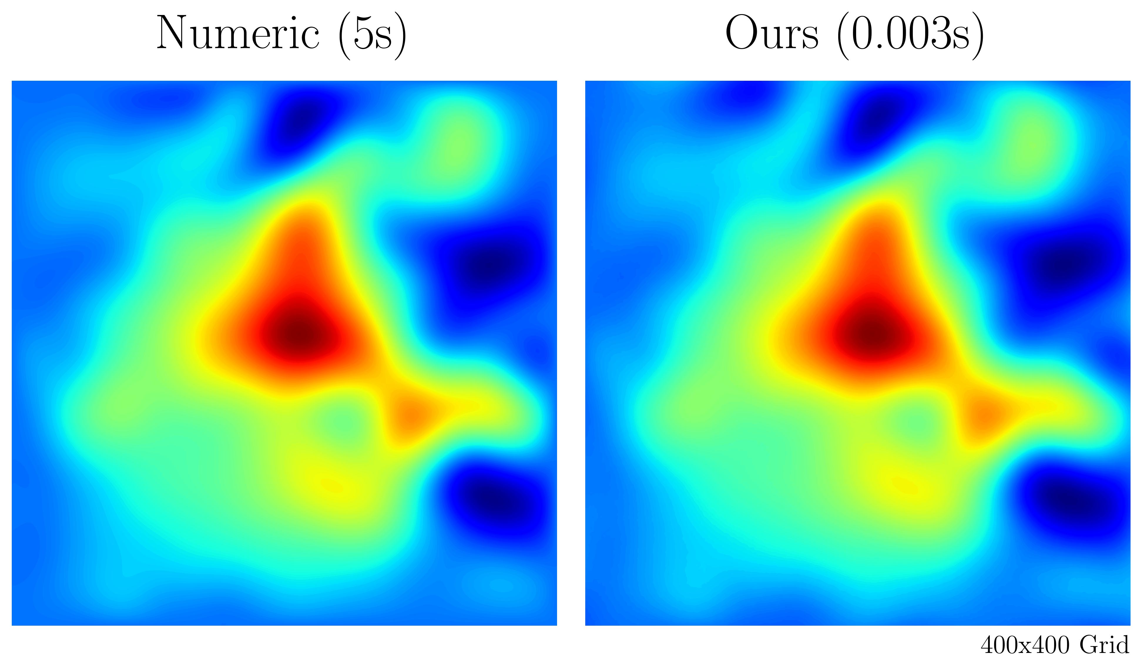
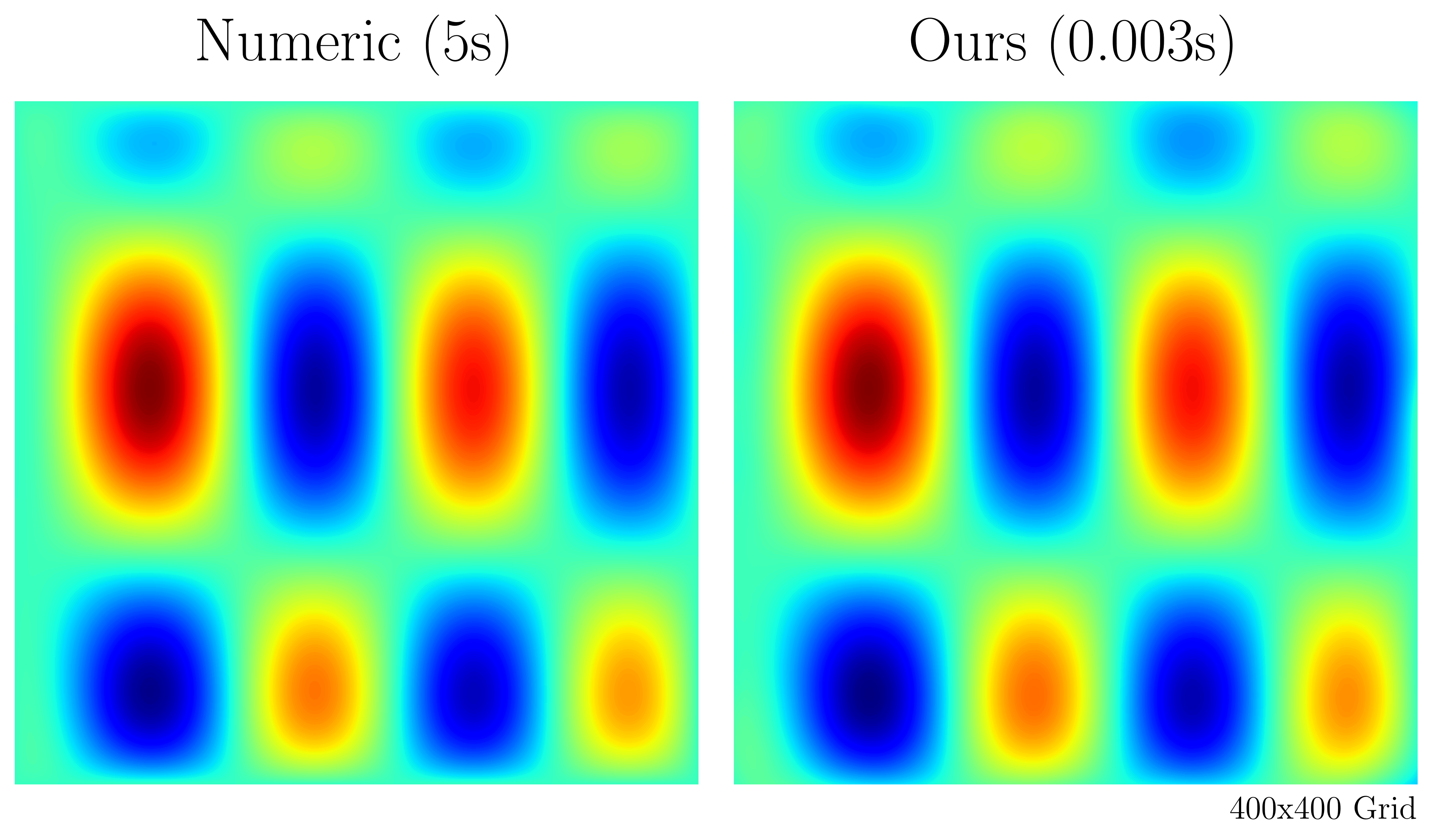
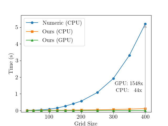
problems. Focusing on the 2D Poisson equation, the
method used in this module shows significant speed improvements over the finite difference
method while maintaining high accuracy in various test scenarios.
The improved efficiency comes from the possibility to pre-compute domain specific steps.
This means, for a given domain, the Poisson equation can be efficiently solved for different source functions and boundary conditions.
The basic usage example below illustrates this.
This approach is therefore only faster, if the Poisson equation needs to solved for the same domain with different source functions and boundary values, e.g. in simulation software.
This module comes with an easy-to-use method for solving arbitrary 2D Poisson problems.
It also includes a numerical solver and an analyzing function to quantify the results.
For visual inspection, the module offers a plotting function.
In its current version this module supports only 2D Poisson problems with Dirichlet boundary conditions.
The boundary conditions should be a constant value.
## Installation
This project is available on PyPI and can be installed with pip.
```bash
pip install fast-poisson-solver
```
Ensure that you have the latest version of pip; if you're unsure, you can upgrade pip with the following command:
```bash
pip install --upgrade pip
```
You might need to use `pip3` instead of `pip`, depending on your system.
## Basic Usage
The Fast Poisson Solver is designed to be highly adaptable and flexible. It can accept a variety of input formats, including lists, numpy arrays, and PyTorch tensors. Please note that currently, only 2D domains are supported.
The solver requires `x` and `y` coordinates for both the PDE domain and the boundary region. The order of these coordinates does not matter. For each pair of `x` and `y` coordinates, the PDE domain needs a value for the source function, and the boundary domain needs a value for the boundary condition.
Once the pre-computation for each domain and boundary region is done, it can be used for unlimited different source functions and boundary condition values.
Here is a basic example:
```python
from fast_poisson_solver import Solver
solver = Solver()
solver.precompute(x_pde, y_pde, x_bc, y_bc)
u_ml, u_ml_pde, u_ml_bc, f_ml, t_ml = solver.solve(f1, u_bc1)
u_ml, u_ml_pde, u_ml_bc, f_ml, t_ml = solver.solve(f2, u_bc2)
u_ml, u_ml_pde, u_ml_bc, f_ml, t_ml = solver.solve(f3, u_bc3)
# ...
```
Please replace x_pde, y_pde, x_bc, y_bc, f, and u_bc with your actual data or variables.
As the approach works best for coordinates that lie between 0 and 1, is it hard limited on this interval.
The order of the coordinates does not matter as long as the `x`, `y` and corresponding source term or value for the boundary condition match.
It is also not important for the coordinates to lie on a grid (Note: The numeric function needs a grid).
For more details see the [Documentation](https://fast-poisson-solver.readthedocs.io/en/latest/)
## Contributing
We warmly welcome contributions to this module.
If you have ideas for improvements, new features, or bug fixes, please feel free to submit a pull request.
We appreciate your support in making this module more useful for everyone.
When making a contribution, please ensure your code adheres to our guidelines, which can also be found in the repository.
## License
Copyright (C) 2023 Matthias Neuwirth
This program is free software: you can redistribute it and/or modify
it under the terms of the GNU General Public License as published by
the Free Software Foundation, either version 3 of the License, or
(at your option) any later version.
This program is distributed in the hope that it will be useful,
but WITHOUT ANY WARRANTY; without even the implied warranty of
MERCHANTABILITY or FITNESS FOR A PARTICULAR PURPOSE. See the
GNU General Public License for more details.
You should have received a copy of the GNU General Public License
along with this program. If not, see .
## Contact
If you encounter any issues while using this module, or if you have suggestions for improvements or new features, please report them to us through the "Issues" tab.
## Roadmap and Future Enhancements
* Dirichlet boundary conditions with multiple values or multiple regions of Dirichlet boundary conditions
* Neuman, Robin, and mixed boundary conditions
* Extend this approach to 1D and 3D or even nD
* Easy to compute force term