https://github.com/mlrichter/receptive_field_analysis_toolbox
A toolbox for receptive field analysis and visualizing neural network architectures
https://github.com/mlrichter/receptive_field_analysis_toolbox
deep-learning hacktoberfest machine-learning neural-architecture-optimization neural-architecture-search neural-networks pytorch receptive-field receptive-field-analysis tensorflow visualization
Last synced: over 1 year ago
JSON representation
A toolbox for receptive field analysis and visualizing neural network architectures
- Host: GitHub
- URL: https://github.com/mlrichter/receptive_field_analysis_toolbox
- Owner: MLRichter
- License: mit
- Created: 2021-12-10T09:26:28.000Z (over 4 years ago)
- Default Branch: main
- Last Pushed: 2025-03-11T17:26:57.000Z (over 1 year ago)
- Last Synced: 2025-03-29T20:07:22.291Z (over 1 year ago)
- Topics: deep-learning, hacktoberfest, machine-learning, neural-architecture-optimization, neural-architecture-search, neural-networks, pytorch, receptive-field, receptive-field-analysis, tensorflow, visualization
- Language: Python
- Homepage:
- Size: 1.35 MB
- Stars: 113
- Watchers: 3
- Forks: 5
- Open Issues: 13
-
Metadata Files:
- Readme: README.md
- Changelog: CHANGELOG.md
- Contributing: CONTRIBUTING.md
- Funding: .github/FUNDING.yml
- License: LICENSE
Awesome Lists containing this project
README
# ReceptiveFieldAnalysisToolbox


This is RFA-Toolbox, a simple and easy-to-use library that allows you to optimize your neural network architectures
using receptive field analysis (RFA) and create graph visualizations of your architecture.
## Installation
Install this via pip:
`pip install rfa_toolbox`
## What is Receptive Field Analysis?
Receptive Field Analysis (RFA) is a simple yet effective way to optimize the efficiency of any neural architecture without
training it.
## Usage
This library allows you to look for certain inefficiencies withing your convolutional neural network setup without
ever training the model.
You can do this simply by importing your architecture into the format of RFA-Toolbox and then use the in-build functions
to visualize your architecture using GraphViz.
The visualization will automatically mark layers predicted to be unproductive red and critical layers, that are potentially unproductive orange.
In edge case scenarios, where the receptive field expands of the boundaries of the image on some but not all tensor-axis, the layer will be marked yellow,
since such a layer is probably not operating and maximum efficiency.
Being able to detect these types of inefficiencies is especially useful if you plan to train your model on resolutions that are substantially lower than the
design-resolution of most models.
As an alternative, you can also use the graph from RFA-Toolbox to hook RFA-toolbox more directly into your program.
### Examples
There are multiple ways to import your model into RFA-Toolbox for analysis, with additional ways being added in future
releases.
#### PyTorch
The simplest way of importing a model is by directly extracting the compute-graph from the PyTorch-implementation of your model.
Here is a simple example:
```python
import torchvision
from rfa_toolbox import create_graph_from_pytorch_model, visualize_architecture
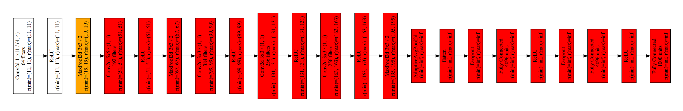
model = torchvision.models.alexnet()
graph = create_graph_from_pytorch_model(model)
visualize_architecture(
graph, f"alexnet_32_pixel", input_res=32
).view()
```
This will create a graph of your model and visualize it using GraphViz and color all layers that are predicted to be
unproductive for an input resolution of 32x32 pixels:
Keep in mind that the Graph is reverse-engineerd from the PyTorch JIT-compiler, therefore no looping-logic is
allowed within the forward pass of the model.
Also, the use of the functional-library for stateful-operations like pooling or convolutional layers is discouraged,
since it can cause malformed graphs during the reverse engineering of the compute graph.
#### Tensorflow / Keras
Similar to the PyTorch-import, models can be imported from TensorFlow as well.
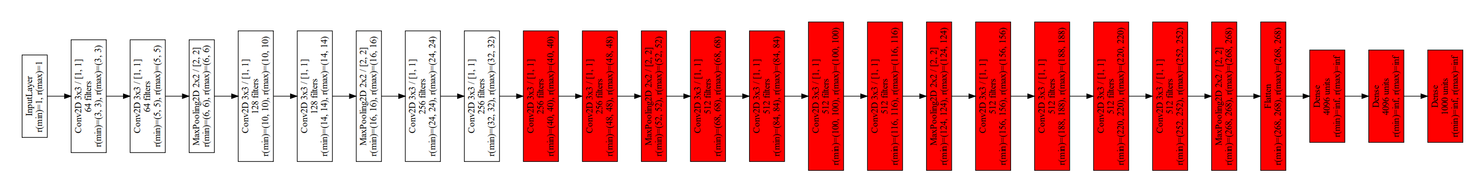
The code below will create a graph of VGG16 and visualize it using GraphViz and color all layers that are predicted to be
unproductive for an input resolution of 32x32 pixels. This is analog to the PyTorch-variant depicted above:
```python
from keras.applications.vgg19 import VGG19
from rfa_toolbox import create_graph_from_tensorflow_model
model = VGG19(include_top=True, weights=None)
graph: EnrichedNetworkNode = create_graph_from_tensorflow_model(model)
visualize_architecture(graph, "VGG16", input_res=32).view()
```
This will create the following visualization:
Currently, only the use of the keras.Model object is supported.
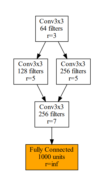
#### Custom
If you are not able to automatically import your model from PyTorch or you just want some visualization, you can
also directly implement the model with the propriatary-Graph-format of RFA-Toolbox.
This is similar to coding a compute-graph in a declarative style like in TensorFlow 1.x.
```python
from rfa_toolbox import visualize_architecture
from rfa_toolbox.graphs import EnrichedNetworkNode, LayerDefinition
conv1 = EnrichedNetworkNode(
name="Conv1",
layer_info=LayerDefinition(
name="Conv3x3",
kernel_size=3, stride_size=1,
filters=64
),
predecessors=[]
)
conv2 = EnrichedNetworkNode(
name="Conv2",
layer_info=LayerDefinition(
name="Conv3x3",
kernel_size=3, stride_size=1,
filters=128
),
predecessors=[conv1]
)
conv3 = EnrichedNetworkNode(
name="Conv3",
layer_info=LayerDefinition(
name="Conv3x3",
kernel_size=3, stride_size=1,
filters=256
),
predecessors=[conv1]
)
conv4 = EnrichedNetworkNode(
name="Conv4",
layer_info=LayerDefinition(
name="Conv3x3",
kernel_size=3, stride_size=1,
filters=256
),
predecessors=[conv2, conv3]
)
out = EnrichedNetworkNode(
name="Softmax",
layer_info=LayerDefinition(
name="Fully Connected",
units=1000
),
predecessors=[conv4]
)
visualize_architecture(
out, f"example_model", input_res=32
).view()
```
This will produce the following graph:
#### Finding the feasible input range of a neural network
With RFA-Toolbox you can also easily determine in which range your input resolution should be in order to allow
the network to use all parameters to solve the problem, which is the most efficient way to operate the model.
```python
import torchvision
from rfa_toolbox import create_graph_from_pytorch_model, input_resolution_range
model = torchvision.models.resnet50()
graph = create_graph_from_pytorch_model(model)
# set filter_all_inf_rf to True, if your model contains Squeeze-And-Excitation-Modules
min_res, max_res = input_resolution_range(graph, filter_all_inf_rf=False) # (75, 75), (427, 427)
print("Mininum Resolution:", min_res, "Maximum Resolution:", max_res)
```
Every resolution below the minimum resolution will result in unproductive layers in the network, due to oversized
receptive field sizes (see next section for details).
Every resolution above the maximum resolution exceeds the maximum receptive field size of any non-fully-connected
layer in the model, which means that potentially patterns exist in the input that the network cannot extract with
its feature-extractor.
### A quick primer on the Receptive Field
To understand how RFA works, we first need to understand what a receptive field is, and it's effect on what the network is learning to detect.
Every layer in a (convolutional) neural network has a receptive field. It can be considered the "field of view" of this layer.
In more precise terms, we define a receptive field as the area influencing the output of a single position of the
convolutional kernel.
Here is a simple, 1-dimensional example:
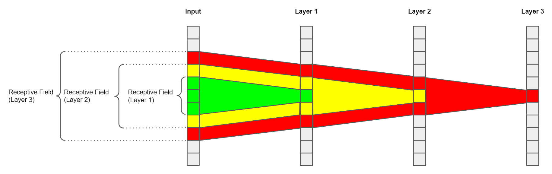
The first layer of this simple architecture can only ever "see" the information the input pixels directly
under its kernel, in this scenario 3 pixels.
Another observation we can make from this example is that the receptive field size is expanding from layer to layer.
This is happening, because the consecutive layers also have kernel sizes greater than 1 pixel, which means that
they combine multiple adjacent positions on the feature map into a single position in their output.
In other words, every consecutive layer adds additional context to each feature map position by expanding the receptive field.
This ultimately allows networks to go from detecting small and simple patterns to big and very complicated ones.
The effective size of the kernel is not the only factor influence the growth of the receptive field size.
Another important factor is the stride size:
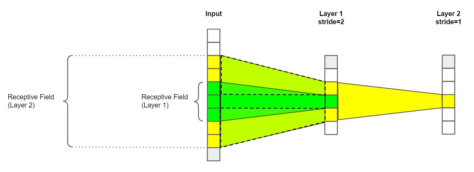
The stride size is the size of the step between the individual kernel positions. Commonly, every possible
position is evaluated, which is not affecting the receptive field size in any way.
When the stride size is greater than one however valid positions of the kernel are skipped, which reduces
the size of the feature map. Since now information on the feature map is now condensed on fewer feature map positions,
the growth of the receptive field is multiplied for future layers.
In real-world architectures, this is typically the case when downsampling layers like convolutions with a stride size of 2
are used.
### Why does the Receptive Field Matter?
At this point you may be wondering why the receptive field of all things is useful for optimizing an
architecture.
The short answer to this is: because it influences where the network can process patterns of a certain size.
Simply speaking each convolutional layer is only able to detect patterns of a certain size because of its receptive field.
Interestingly this also means that there is an upper limit to the usefulness of expanding the receptive field.
At the latest, this is the case when the receptive field of a layer is BIGGER than the input image, since no novel
context can be added at this point.
For convolutional layers this is a problem, because layers past this "Border Layer" now lack the primary mechenism convolutional layers
use to improve the intermediate representation of the data, making these layers unproductive.
If you are interested in the details of this phenomenon I recommend that you read these:
- [(Input) Size Matters for Convolutional Neural Network Classifier](https://link.springer.com/chapter/10.1007/978-3-030-86340-1_11)
- [Should You Go Deeper? Optimizing Convolutional Neural Network Architectures without Training](https://arxiv.org/abs/2106.12307)
(published at the 20th IEEE International Conference for Machine Learning Application - ICMLA)
### Optimizing Architectures using Receptive Field Analysis
So far, we learned that the expansion of the receptive field is the primary mechanism for improving
the intermediate solution utilized by convolutional layers.
At the point where this is no longer possible, layers are not able to contribute to the quality of the output of the model
and become unproductive.
We refer to these layers as unproductive layers. Layers who advance the receptive field sizes beyond the input resolution
are referred to as critical layers.
Critical layers are not necessarily unproductive, since they are still able to incorporate some novel context into the data,
depending on how large the receptive field size of the input is.
Of course, being able to predict why and which layer will become dead weight during training is highly useful, since
we can now adjust the design of the architecture to fit our input resolution better without spending time on training models.
Depending on the requirements, we may choose to emphasize efficiency by primarily removing unproductive layers. Another
option is to focus on predictive performance by making the unproductive layers productive again.
We now illustrate how you may choose to optimize an architecture on a simple example:
Let's take the ResNet architecture, which is a very popular CNN-model.
We want to train ResNet18 on ResizedImageNet16, which has a 16 pixel input resolution.
When we apply Receptive Field Analysis, we can see that most convolutional layers will in fact not contribute
to the inference process (unproductive layers marked red, probable unproductive layers marked orange):
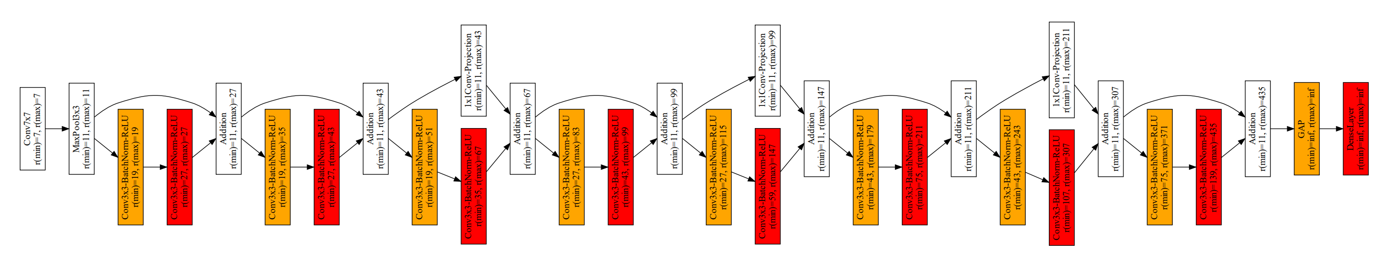
We can clearly see that most of the network's layers will not contribute anything useful to the quality of the output, since
their receptive field sizes are too large.
From here on we have multiple ways of optimizing the setup.
Of course, we can simply increase the resolution, to involve more layers in the inference process, but that is usually
very expensive from a computational point of view.
In the first scenario, we are not interested in increasing the predictive performance of the model, we simply want to save
computational resources. We reduce the kernel size of the
first layer to 3x3 from 7x7.
This change allows the first three building blocks to contribute more to
the quality of the prediction, since no layer is predicted to be unproductive.
We then simply replace the remaining building blocks with a simple output head.
This new architecture then looks like this:
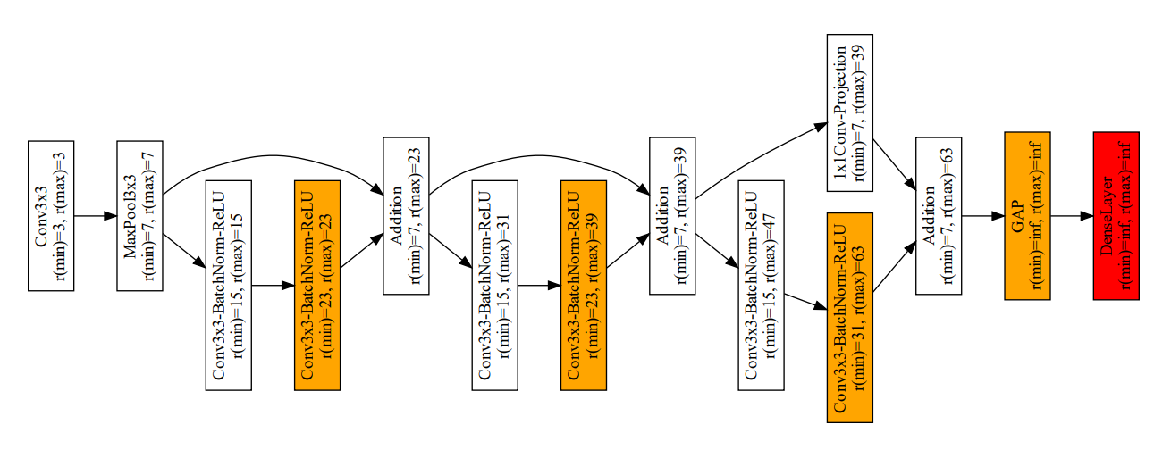
Note that all previously unproductive layers are now either removed or only marked as "critical", which
is generally not a big problem, since the receptive field size is "reset" by the receptive field size
after each building block.
Also note that fully connected layers are always marked as critical or unproductive, since they
technically have an infinite receptive field size.
The resulting architecture achieves slightly better predictive performance as
the original architecture, but with substantially lower computational cost.
In this case we save approx. 80% of the computational cost and improve the predictive performance slightly
from 17% to 18%.
In another scenario we may not be satisfied with the predictive performance.
In other words, we want to make use of the underutilized parameters of the network
by turning all unproductive layers into productive layers.
We achieve this by changing their receptive field sizes.
The biggest lever when it comes to changing the receptive field size is always the quantity of downsampling layers.
Downsampling layers have a multiplicative effect on the growth of the receptive field for all consecutive layers.
We can exploit this by simply removing the MaxPooling layer, which is the second layer of the original
architecture.
We also reduce the kernel size of the first layer to 3x3 from 7x7, and it's stride size to 1.
This drastically reduces the receptive field sizes of the entire architecture, making most layers productive again.
We address the remaining unproductive layers to by removing the final downsampling layer and distributing the building
blocks as evenly as possible among the three stages between the remaining downsampling layers.
The resulting architecture now looks like this:
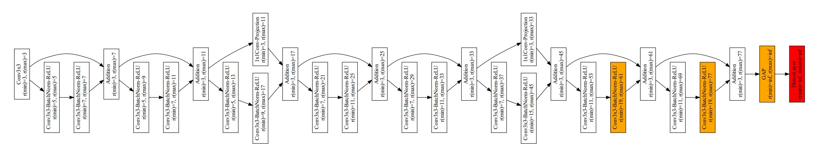
The architecture now no longer has unproductive layers in their building blocks and only 2 critical layers.
This improved architecture also achieves 34% Top1-Accuracy in ResizedImageNet16 instead of the 17% of the original architecture.
However, this improvement comes at a price, since the removed downsampling layers have a negative impact on the computations
required to process an image, which increases by roughly a factor of 8.
In any way, RFAToolbox allows you to optimize your convolutional neural network architectures
for efficiency, performance or a sweetspot between the two without the need for long-running trial-and-error sessions.
## Citation
If you use ReceptiveFieldAnalysisToolbox for your publication, please cite [1] and [2].
[1] M.L. Richter, J. Schöning, A. Wiedenroth & U. Krumnack. Should You Go Deeper? Optimizing Convolutional Neural Network Architectures without Training. In International Conference On Machine Learning And Applications (ICMLA) 2021. IEEE.
[2] M.L. Richter, J. Schöning, A. Wiedenroth & U. Krumnack. Receptive Field Analysis for Optimizing Convolutional Neural Network Architectures Without Training. In Deep Learning Applications 2022. Springer (InPress).
## Credits
This package was created with
[Cookiecutter](https://github.com/audreyr/cookiecutter) and the
[browniebroke/cookiecutter-pypackage](https://github.com/browniebroke/cookiecutter-pypackage)
project template.