https://github.com/mschauer/pointprocessinference.jl
Statistical inference for Poisson Processes
https://github.com/mschauer/pointprocessinference.jl
Last synced: 9 months ago
JSON representation
Statistical inference for Poisson Processes
- Host: GitHub
- URL: https://github.com/mschauer/pointprocessinference.jl
- Owner: mschauer
- Created: 2019-02-28T14:49:27.000Z (over 7 years ago)
- Default Branch: master
- Last Pushed: 2020-12-16T12:28:20.000Z (over 5 years ago)
- Last Synced: 2025-08-13T21:42:56.055Z (11 months ago)
- Language: Julia
- Size: 1.94 MB
- Stars: 7
- Watchers: 3
- Forks: 4
- Open Issues: 3
-
Metadata Files:
- Readme: README.md
Awesome Lists containing this project
README
[pkgeval-img]: https://juliaci.github.io/NanosoldierReports/pkgeval_badges/P/PointProcessInference.svg
[pkgeval-url]: https://juliaci.github.io/NanosoldierReports/pkgeval_badges/report.html
[![][pkgeval-img]][pkgeval-url]
[](https://travis-ci.org/mschauer/PointProcessInference.jl)
# PointProcessInference.jl
Fast and scalable non-parametric Bayesian inference for Poisson point processes
## Introduction
Poisson point processes are among the basic modelling tools in many areas. Their probabilistic properties are determined by their intensity function, the density *λ*.
This Julia package implements our non-parametric Bayesian approach to estimation of the intensity function *λ* for univariate Poisson point processes. For full details see our preprint
- S. Gugushvili, M. Schauer, F. van der Meulen, and P. Spreij. Fast and scalable non-parametric Bayesian inference for Poisson point processes. __[arXiv:1804.03616 [stat.ME]](https://arxiv.org/abs/1804.03616)__, 2018.
Intuitively, a univariate Poisson point processes *X*, also called a non-homogeneous Poisson process, can be thought of as random
scattering of points in the time interval *[0,T]*, where the way the scattering occurs is determined by the intensity function *λ*.
An example is the ordinary Poisson process, for which the intensity *λ* is constant.
## Methodology
We infer the intensity function *λ* in a non-parametric fashion. The function *λ* is a priori modelled as piecewise constant. This is even more natural, if the data have been already binned,
as is often the case in, e.g., astronomy. Thus, fix a positive integer *N* and a grid *b* of points `b[1] == 0`, `b[N] == T` on the interval *[0,T]*, for instance a uniform grid.
The intensity *λ* is then modelled as
`λ(x) = ψ[k]` for `b[k] <= x < b[k+1]`.
Now we postulate that a priori the coefficients *ψ* form a Gamma Markov chain (GMC). As explained in our preprint, this prior induces smoothing across the coefficients *ψ*, and leads to conjugate posterior computations
via the Gibbs sampler. The data-generating intensity is not assumed to be necessarily piecewise constant. Our methodology provides both a point estimate of the intensity function (posterior mean) and uncertainty quantification via marginal credible bands; see the examples below.
## Installation
Change julia into the package manager mode by hitting `]`. Then run the command `add PointProcessInference`.
```
pkg> add PointProcessInference
```
## Usage
In the following example we load the UK coal mining disasters data and
performs its statistical analysis via the Poisson point process.
```
using PointProcessInference
using Random
Random.seed!(1234) # set RNG
observations, parameters, λinfo = PointProcessInference.loadexample("coal")
res = PointProcessInference.inference(observations; parameters...)
```
The main procedure has signature
```julia
PointProcessInference.inference(observations; title = "Poisson process", T = 1.0, n = 1, ...)
```
where `observations` is the sorted vector of Poisson event times, `T` is the endpoint of the time interval considered, and if
`observations` is an aggregate of `n` different independent observations (say aggregated for `n` days), this can be indicated by the parameter `n > 1`. A full list of parameters is as follows:
```julia
function inference(observations;
title = "Poisson process", # optional caption for mcmc run
summaryfile = nothing, # path to summary file or nothing
T0 = 0.0, # start time
T = maximum(observations), # end time
n = 1, # number of aggregated samples in `observations`
N = min(length(observations)÷4, 50), # number of bins
samples = 1:1:30000, # run for `i in 1:last(samples)` iterations, save coefficients if `i ∈ samples`
α1 = 0.1, β1 = 0.1, # parameters for Gamma Markov chain
Π = Exponential(10), # prior on alpha
τ = 0.7, # Set scale for random walk update on log(α)
αind = 0.1, βind = 0.1, # parameters for the independent Gamma prior
emp_bayes = false, # estimate βind using empirical Bayes
verbose = true
)
```
Iterates of *ψ* are the rows of the matrix
```julia
res.ψ
```
## High-quality plots
For high quality plotting, the package has a script `process-output-simple.jl` that visualizes
the results with the help of `R` and `ggplot2`.
After installing the additional dependencies
```
pkg> add RCall
pkg> add DataFrames
```
include the script (it is located in the `contrib` folder, the location can be retrieved by calling `PointProcessInference.plotscript()`)
```
include(PointProcessInference.plotscript())
plotposterior(res)
```
The script starts `ggplot2` with `RCall`, and `plotposterior` expects as its argument the result `res` returned from `inference`. For computing the posterior summary measures, the first half of the MCMC iterates is treated as burnin samples.
## Example 1
Here, we generate data from a nonhomogeneous Poissson process as follows:
```julia
λ0(x) = (20 + 8*cos(x))
λ0max = 28
obs = PointProcessInference.samplepoisson(λ0, λ0max, 0, 10)
```
The nonparametric estimator is obtained by running
```julia
res = PointProcessInference.inference(obs)
```
Finally, a default graph is obtained by
```julia
include(PointProcessInference.plotscript())
plotposterior(res)
```
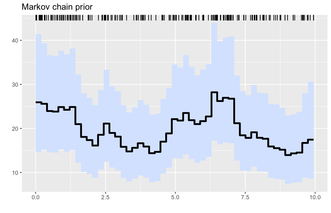
* Illustration: Intensity estimation for the generated data in example 1. The data are displayed via the rug plot in the upper margin of the plot, the posterior mean is given by a solid black line, while a 95% marginal credible band is shaded in light blue.
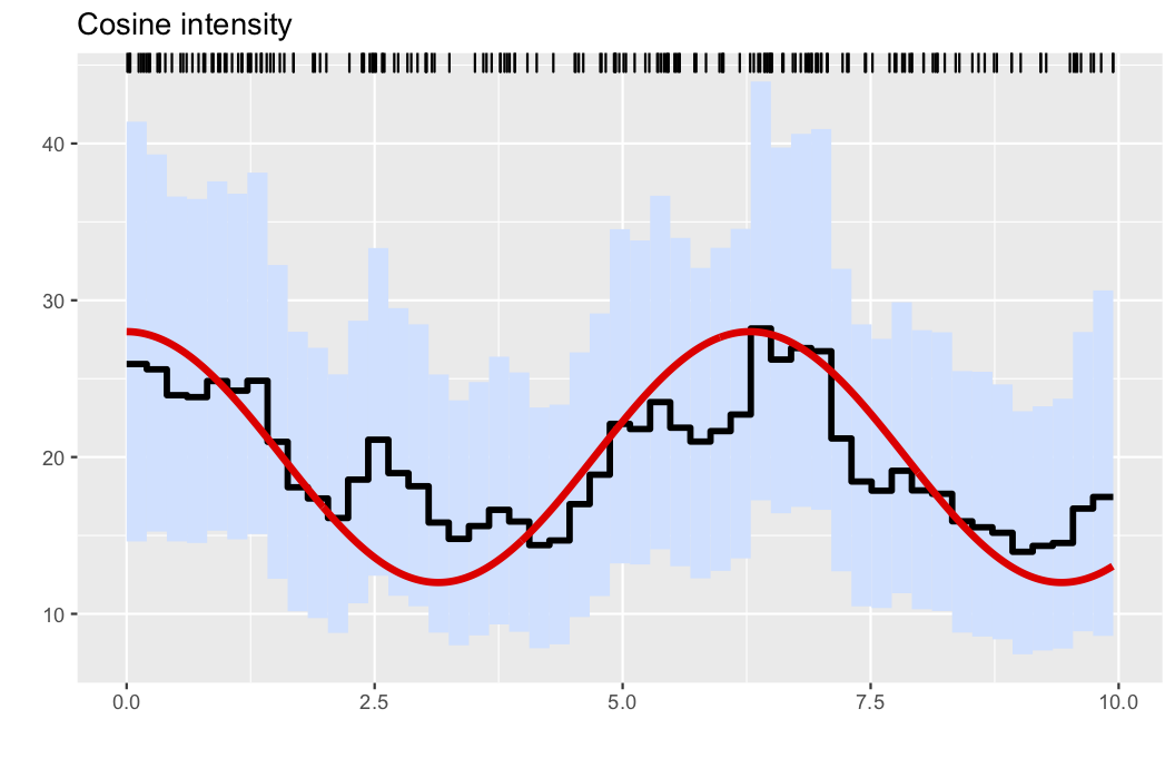
A slightly refined plot, where the true intensity is added to the figure can be obtained by passing the data-generating intensity function as an extra argument.
```julia
plotposterior(res;figtitle="Cosine intensity", λ=λ0)
```
This results in the plot
## Example 2
Here, we analyse the well-known coal mining disasters data set.
```julia
observations, parameters, λinfo = PointProcessInference.loadexample("coal")
res = PointProcessInference.inference(observations)
plotposterior(res)
```
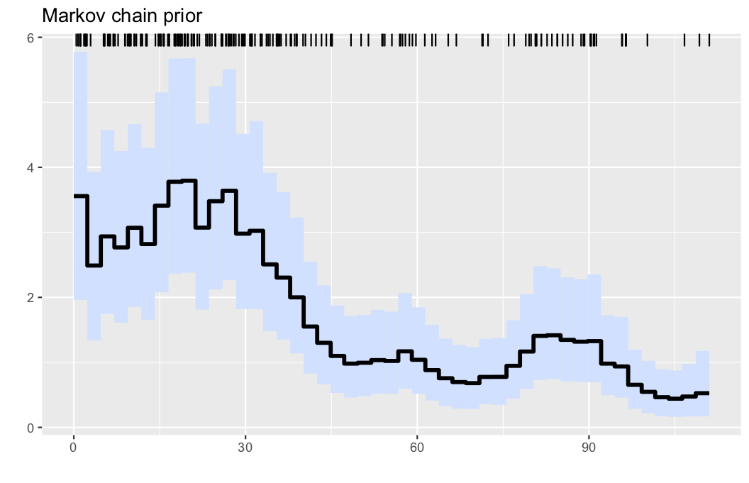
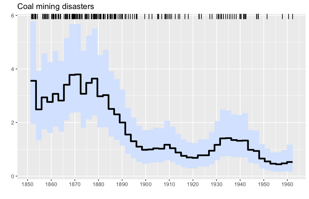
* Illustration: Intensity estimation for the UK coal mining disasters data (1851-1962). The data are displayed via the rug plot in the upper margin of the plot, the posterior mean is given by a solid black line, while a 95% marginal credible band is shaded in light blue.
The horizontal tickmarks can be adjusted, as the offset date of the data, which is March 15, 1851 in this case.
```julia
start = 1851+(28+31+15)/365
plotposterior(res; figtitle="Coal mining disasters", offset = start,hortics=1850:10:1960)
```
## Citing the package
If you use the package in your work, we encourage you to cite it using the following BibTeX code:
```
@misc{pppjl,
title = { {PointProcessInference 0.1.0 -- Code and Julia package accompanying the article ``Gugushvili, van der Meulen, Schauer, Spreij (2018): Fast and scalable non-parametric Bayesian inference for Poisson point processes" ({http://arxiv.org/abs/1804.03616})} },
author = {Gugushvili, Shota and van der Meulen, Frank and Schauer, Moritz and Spreij, Peter},
year = {2019},
doi = {10.5281/zenodo.2591395},
url = {https://doi.org/10.5281/zenodo.2591395},
}
```