https://github.com/nazanin1369/artificial-neural-network
https://github.com/nazanin1369/artificial-neural-network
artificial-neural-networks machine-learning neurons perceptron
Last synced: 8 months ago
JSON representation
- Host: GitHub
- URL: https://github.com/nazanin1369/artificial-neural-network
- Owner: Nazanin1369
- Created: 2016-08-22T00:18:32.000Z (about 9 years ago)
- Default Branch: master
- Last Pushed: 2016-08-24T07:17:50.000Z (about 9 years ago)
- Last Synced: 2025-01-07T20:50:22.343Z (9 months ago)
- Topics: artificial-neural-networks, machine-learning, neurons, perceptron
- Language: Python
- Size: 11.7 KB
- Stars: 0
- Watchers: 1
- Forks: 1
- Open Issues: 0
-
Metadata Files:
- Readme: readme.md
Awesome Lists containing this project
README
### Implementation of Perceptron in Python
### Project Overview
The first perceptron algorithm was implemented in 1950 in custom hardware at the _Cornell Aeronautical Laboratory_ by _Frank Rosenblatt_.
The perceptron was intended to be a machine, rather than a program, and while its first implementation was in software for the IBM 704, it was subsequently implemented in custom-built hardware as the "Mark 1 perceptron". This machine was designed for image recognition: it had an array of 400 photocells, randomly connected to the "neurons". Weights were encoded in potentiometers, and weight updates during learning were performed by electric motors.
Although the perceptron was initially promising, it was quickly proved that perceptrons could not be trained to recognize many classes of patterns. This led to the field of neural network research stagnating for many years.
As we will see later, the adaline is an improvement of the perceptron algorithm and offers a good opportunity to learn about a popular optimization algorithm in machine learning: _gradient descent_.
##### Artificial Neuron
The idea of artificial neuron first proposed by _Warren McCulloch_ and _Walter Pitts_ in 1943. The model was specifically targeted as a computational model of the _"nerve net"_ in the brain.
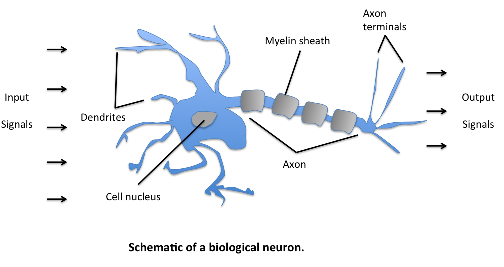
Neurons can be understood as the subunits of a neural network in a biological brain. As illustrated below, the signals of variable wights arrive at the dendrites. Those input signals are then accumulated in the cell body of the neuron, and if the accumulated signal exceeds a certain threshold, a output signal is generated that which will be passed on by the axon.
One important and pioneering artificial neural network that used the _linear threshold function_ was the perceptron, developed by _Frank Rosenblatt_. This model already considered more flexible weight values in the neurons, and was used in machines with adaptive capabilities.
##### Frank Rosenblatt Single-layer perceptrons
Single-layer perceptrons use Heaviside step function as activation function. Heaviside step function is a discontinuous function whose value is zero for negative argument and one for positive argument as you see below.

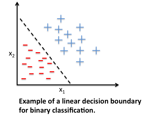
Perceptron unit is pretty powerful in sense of linear classification. Perceptrons supposed to learn the weight value and make a decision whether to activate or not. In machine learning context perceptron can be useful to categorize a set of input or samples into one class or another. Single-layer perceptron belongs to supervised learning since the task is to predict to which of two possible categories a certain data point belongs based on a set of input variables.
For multilayer perceptrons, where a hidden layer exists, more sophisticated algorithms such as _backpropagation_ must be used. Alternatively, methods such as the _delta rule_ can be used if the function is non-linear and differentiable.
##### Perceptron Learning Rule
Learning rule is a procedure for modifying the weights and biases of a network.
The purpose of the learning rule is to train the network to perform some task. There are many types of neural network learning rules. They fall into three broad categories: supervised learning, unsupervised learning and reinforcement (or graded) learning.
Here we will go over the learning rule for single-layer networks which is in supervised learning category.
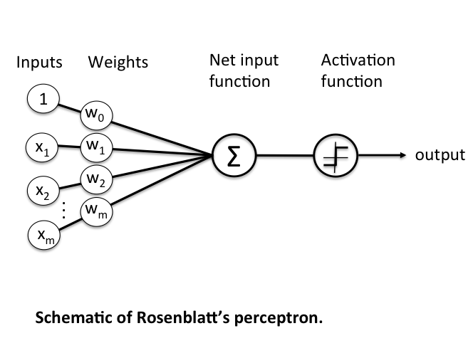
A perceptron get's set of inputs and weights and pass those along to Net input function. Net input function will sum the multiplication of inputs and weights and pass the result to activation function. Activation function is an step function which will produce two different outputs based on the threshold. The idea behind the threshold was to mimic how actual neurons in brain work, they fire or don't.
The learning rule in the repetition of steps above to produce an appropriate output.
So the learning rule can be summarized into following steps:
summarized by the following steps:
1- Initialize the weights to 0 or small random numbers.
2- For each training sample x(i)x(i):
* Calculate the output value.
* Update the weights.
The output value is the class label predicted by the unit step function that we defined earlier (output =g(z)=g(z)) and the weight update can be written more formally as
```
wj:=wj+Δwjwj:=wj+Δwj
```
The value for updating the weights at each increment is calculated by the learning rule
```
Δwj=η(target(i)−output(i))x(i)j
Δwj=η(target(i)−output(i))xj(i)
```
where η is the learning rate (a constant between 0.0 and 1.0), “target” is the true class label, and the “output” is the predicted class label.
It is important to note that all weights in the weight vector are being updated simultaneously. Concretely, for a 2-dimensional dataset, we would write the update as:
```
Δw0=η(target(i)−output(i))Δw0=η(target(i)−output(i))
Δw1=η(target(i)−output(i))x(i)1Δw1=η(target(i)−output(i))x1(i)
Δw2=η(target(i)−output(i))x(i)2Δw2=η(target(i)−output(i))x2(i)
```
Before we implement the perceptron rule in Python, let us make a simple thought experiment to illustrate how beautifully simple this learning rule really is. In the two scenarios where the perceptron predicts the class label correctly, the weights remain unchanged:
```
Δwj=η(−1(i)−−1(i))x(i)j=0Δwj=η(−1(i)−−1(i))xj(i)=0
Δwj=η(1(i)−1(i))x(i)j=0Δwj=η(1(i)−1(i))xj(i)=0
```
However, in case of a wrong prediction, the weights are being “pushed” towards the direction of the positive or negative target class, respectively:
```
Δwj=η(1(i)−−1(i))x(i)j=η(2)x(i)jΔwj=η(1(i)−−1(i))xj(i)=η(2)xj(i)
Δwj=η(−1(i)−1(i))x(i)j=η(−2)x(i)jΔwj=η(−1(i)−1(i))xj(i)=η(−2)xj(i)
```
It is important to note that the convergence of the perceptron is only guaranteed if the two classes are linearly separable. If the two classes can’t be separated by a linear decision boundary, we can set a maximum number of passes over the training dataset (“epochs”) and/or a threshold for the number of tolerated misclassifications.