https://github.com/palmstudio/biomech
Biomechanical deformation model (torsion + bending)
https://github.com/palmstudio/biomech
Last synced: 2 months ago
JSON representation
Biomechanical deformation model (torsion + bending)
- Host: GitHub
- URL: https://github.com/palmstudio/biomech
- Owner: PalmStudio
- License: mit
- Created: 2020-09-14T13:44:46.000Z (over 4 years ago)
- Default Branch: master
- Last Pushed: 2021-07-15T08:41:45.000Z (almost 4 years ago)
- Last Synced: 2025-01-28T19:47:31.053Z (4 months ago)
- Language: R
- Homepage: https://palmstudio.github.io/biomech/
- Size: 1.83 MB
- Stars: 0
- Watchers: 3
- Forks: 0
- Open Issues: 0
-
Metadata Files:
- Readme: README.Rmd
- License: LICENSE
Awesome Lists containing this project
README
---
output: github_document
bibliography: references.bib
---
```{r, include = FALSE}
knitr::opts_chunk$set(
collapse = TRUE,
comment = "#>",
fig.path = "man/figures/README-",
out.width = "100%"
)
```
# biomech
[](https://github.com/PalmStudio/biomech/actions)
`biomech` aims at computing bending and torsion of beams following the Euler-Bernoulli beam theory. It is specifically designed to be applied on
tree branches (or e.g. palm leaves), but can be applied to any other beam-shaped structure.
## Table of Contents
* [1. Installation](#1-installation)
* [2. Examples](#2-examples)
* [2.1 Example field data](#21-example-field-data)
* [2.1.1 Presentation](#211-presentation)
* [2.1.2 Un-bending](#211-un-bending)
* [2.2 Bending model](#22-bending-model)
* [2.3 Plotting](#23-plotting)
* [2.4 Optimization](#24-optimization)
* [3. References](#3-references)
## 1. Installation
You can install biomech from [GitHub](https://github.com/) with:
``` r
# install.packages("devtools")
devtools::install_github("PalmStudio/biomech")
```
## 2. Examples
The bending function (`bend()`) uses two parameters: the elastic modulus, and the shear modulus. A good introduction to these concepts is available on [wikipedia](https://en.wikipedia.org/wiki/Euler%E2%80%93Bernoulli_beam_theory)
In our examples, these parameters are unknown at first, but they can be computed from field data.
### 2.1 Example field data
#### 2.1.1 Presentation
Our field data consist on measurements made along the leaf of a palm plant. The leaf is discretized into 5 segments. each segment is defined by a single point at the beginning of the segment representing its cross-section, with attributes such as its dimensions (width, height) and shape (=`type`), the distance from the last point to the current point, the inclination and torsion at the first point, the x, y and z positions of the point (used to cross-validate), the mass of the rachis and of the leaflets on the right and on the left separately.
Here is a little depiction of the information:
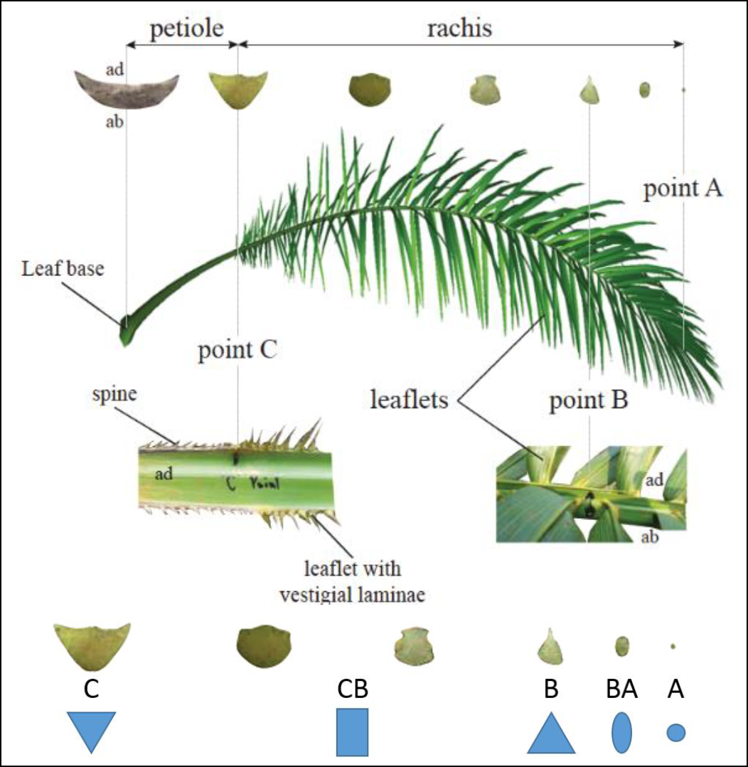
See [@perezAnalyzingModellingGenetic2017] for more information about the subject.
The example field data is available from the package and can be read using:
```{r example}
library(biomech)
file_path = system.file("extdata/6_EW01.22_17_kanan.txt", package = "biomech")
field_data = read_mat(file_path)
```
Here is what it looks like:
```{r echo=FALSE}
field_data
```
#### 2.1.2 Un-bending
We can use the field data to try our bending model. But first, it must be "un-bent" back to a straight line. This is made using `unbend()`, such as:
```{r}
# Un-bending the field measurements:
df_unbent = unbend(field_data)
```
### 2.2 Bending model
We can use `bend()` to bend a straight beam providing initial values and known elastic and shear modulus.
We can try it out on our example leaf data. But first, we have to compute a variable that is missing from our `df_unbent` data.frame: the distance of application of the mass of the leaflets on the right and left sides of each segment. We can approximate this using a sine function:
```{r}
# Adding the distance of application of the left and right weight (leaflets):
df_unbent$distance_application = distance_weight_sine(df_unbent$x)
```
Know we're ready to go with our model, using some expert knowledge to estimate the elastic and shear modulus:
```{r}
# (Re-)computing the deformation:
df_bent = bend(df_unbent, elastic_modulus = 2000, shear_modulus = 400)
```
### 2.3 Plotting
We can now plot the results using `plot_bending()`. We want to compare the observed data with the simulated data. We also want to check if the straight line was right. Let's put all three on a single plot:
```{r}
plot_bending(Observed = field_data, "Un-Bent obs." = df_unbent, Modeled = df_bent)
```
We can even make a 3d plots using `plot_bent_3d()`:
```{r eval=FALSE}
plot_bending_3d(Observed = field_data, "Un-Bent obs." = df_unbent, Modeled = df_bent)
```
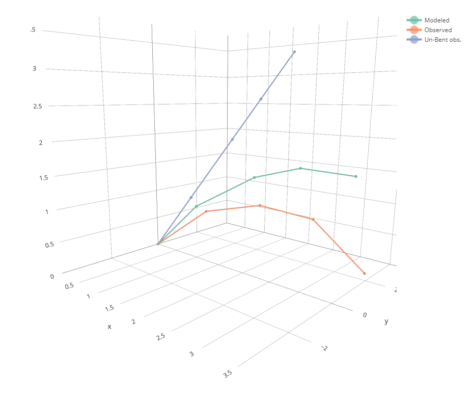
OK, not bad. But the adjustment is not really that close to the measurement.
### 2.4 Optimization
`optimize_bend()` can help us find out the right values for both our parameters:
```{r eval=TRUE}
params = optimize_bend(field_data, type = "all")
```
```{r include=FALSE}
# params = list(elastic_modulus = 1209.396, shear_modulus = 67.44096)
```
Here are our optimized values:
```{r}
params
```
And here is a the resulting plot:
```{r}
df_bent_optim = bend(df_unbent, elastic_modulus = params$elastic_modulus,
shear_modulus = params$shear_modulus)
plot_bending(Observed = field_data, "Un-Bent obs." = df_unbent,
Modeled = df_bent,
"Modeled (optimized)" = df_bent_optim)
```
## 3. References