https://github.com/pbenner/double-descent
Simple examples of double descent (benign overfitting)
https://github.com/pbenner/double-descent
Last synced: about 1 month ago
JSON representation
Simple examples of double descent (benign overfitting)
- Host: GitHub
- URL: https://github.com/pbenner/double-descent
- Owner: pbenner
- Created: 2022-05-29T11:02:30.000Z (about 4 years ago)
- Default Branch: master
- Last Pushed: 2022-05-30T14:01:10.000Z (about 4 years ago)
- Last Synced: 2025-01-12T20:21:51.520Z (over 1 year ago)
- Language: Jupyter Notebook
- Size: 298 KB
- Stars: 2
- Watchers: 2
- Forks: 0
- Open Issues: 0
-
Metadata Files:
- Readme: README.md
Awesome Lists containing this project
README
Examples of Double Descent
## Import python packages
``` python
import numpy as np
import matplotlib.pyplot as plt
from numpy.random import default_rng
from sklearn.model_selection import LeaveOneOut, GridSearchCV
from sklearn.linear_model import LinearRegression
```
------------------------------------------------------------------------
## Intuition behind double descent
``` python
import matplotlib.pyplot as plt
%matplotlib inline
plt.axis('off')
plt.arrow(0, 0, 1.0, 0.0, head_width=0.05, head_length=0.1, fc='k', ec='k'); plt.figtext(0.90, 0.25, r'$f_1$', fontsize=26)
plt.arrow(0, 0, 0.4, 0.6, head_width=0.05, head_length=0.1, fc='k', ec='k'); plt.figtext(0.50, 0.70, r'$f_2$', fontsize=26)
plt.arrow(0, 0, 0.9, -0.2, head_width=0.05, head_length=0.1, fc='tab:blue' , ec='tab:blue' ); plt.figtext(0.83, 0.10, r'$f_3$', fontsize=26)
plt.arrow(0, 0, 0.0, 0.8, head_width=0.05, head_length=0.1, fc='tab:blue' , ec='tab:blue' ); plt.figtext(0.10, 0.90, r'$f_4$', fontsize=26)
plt.arrow(0, 0, 0.7, 0.4, head_width=0.05, head_length=0.1, fc='tab:orange', ec='tab:orange'); plt.figtext(0.70, 0.55, r'$y$', fontsize=26)
plt.show()
```

According to the above image, we define four feature vectors
^\top"),
^\top"),
^\top"),
and
^\top").
The response
^\top")
lies in the plane defined by the first two feature vectors
 and
.
``` python
f1 = np.array([1.0, 0.0, 0.0])
f2 = np.array([0.0, 1.0, 0.0])
f3 = np.array([1.0, -0.2, 0.0])
f4 = np.array([0.0, 0.0, 1.0])
y = np.array([1.0, 1.0, 0.0])
```
We study the length of the OLS solution, which for
 is
given by the parameter vector with minimum
-norm.
``` python
def OLSnorm(X, y):
return np.linalg.norm(np.linalg.pinv(X.T@X)@X.T@y)
```
As baseline, we begin with the OLS solution if we are only given
 and
:
``` python
OLSnorm(np.array([f1, f2]).T, y)
```
1.4142135623730951
The length of the solution decreases if we add another feature vector to
X:
``` python
OLSnorm(np.array([f1, f2, f3]).T, y)
```
1.2985663286116427
However, this is only the case if the feature vector is correlated with
:
``` python
OLSnorm(np.array([f1, f2, f4]).T, y)
```
1.4142135623730951
------------------------------------------------------------------------
## Data set
``` python
data = np.array([
0.001399613, -0.23436656,
0.971629779, 0.64689524,
0.579119475, -0.92635765,
0.335693937, 0.13000706,
0.736736086, -0.89294863,
0.492572335, 0.33854780,
0.737133774, -1.24171910,
0.563693769, -0.22523318,
0.877603280, -0.12962722,
0.141426545, 0.37632006,
0.307203910, 0.30299077,
0.024509308, -0.21162739,
0.843665029, -0.76468719,
0.771206067, -0.90455412,
0.149670258, 0.77097952,
0.359605608, 0.56466366,
0.049612895, 0.18897607,
0.409898906, 0.32531750,
0.935457898, -0.78703491,
0.149476207, 0.80585375,
0.234315216, 0.62944986,
0.455297119, 0.02353327,
0.102696671, 0.27621694,
0.715372314, -1.20379729,
0.681745393, -0.83059624 ]).reshape(25,2)
y = data[:,1]
X = data[:,0:1]
plt.scatter(X[:,0], y)
plt.show()
```

------------------------------------------------------------------------
## Linear regressor class
We use the following linear regressor class for all double descent
examples. It takes only the first
 columns from the
feature matrix  and
computes the minimum
-norm
solution when
.
``` python
class MyRidgeRegressor:
def __init__(self, p=3, alpha=0.0):
self.p = p
self.theta = None
self.alpha = alpha
def fit(self, F, y):
F = F[:, 0:self.p]
self.theta = np.linalg.pinv(F.transpose()@F + self.alpha*np.identity(F.shape[1]))@F.transpose()@y
def predict(self, F):
F = F[:, 0:self.p]
return F@self.theta
def set_params(self, **parameters):
for parameter, value in parameters.items():
setattr(self, parameter, value)
return self
def get_params(self, deep=True):
return {"p" : self.p, "alpha" : self.alpha}
```
------------------------------------------------------------------------
## Model evaluation
``` python
def evaluate_model(fg, X, y, n, ps, runs=10):
estimator = MyRidgeRegressor()
result = None
for i in range(runs):
F, y = fg(X, y, n, np.max(ps), random_state=i)
clf = GridSearchCV(estimator=estimator,
param_grid=[{ 'p': list(ps) }],
cv=LeaveOneOut(),
scoring="neg_mean_squared_error")
clf.fit(F, y)
if result is None:
result = -clf.cv_results_['mean_test_score']
else:
result += -clf.cv_results_['mean_test_score']
return result / runs
```
------------------------------------------------------------------------
## 1 Random features
This example of double descent uses covariates generated from a
multivariate normal distribution, i.e. the
-th column of X is given
by

")
In order to obtain a double descent phenomenon, we need that some
 are highly
correlated with  and the
remaining features are uncorrelated. Hence, we define
and generate observations
 according to the linear
model

where
").
``` python
class RandomFeatures():
def __init__(self, scale = 1):
self.scale = scale
def __call__(self, X, y, n, p, random_state=42):
rng = default_rng(seed=random_state)
mu = np.repeat(0, n)
sigma = np.identity(n)
F = rng.multivariate_normal(mu, sigma, size=p).T
theta = np.array([ 1/(j+1) for j in range(p) ])
y = F@theta + rng.normal(0, self.scale, size=n)
return F, y
```
------------------------------------------------------------------------
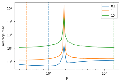
## Results
``` python
ps = range(3, 151)
scales = [0.1, 1, 10]
result = [ evaluate_model(RandomFeatures(scale=scale), None, None, 20, ps, runs=100) for scale in scales ]
result = np.array(result)
```
``` python
p = plt.plot(ps, result.T)
[ plt.axvline(x=ps[np.argmin(result[i])], color=p[i].get_color(), alpha=0.5, linestyle='--') for i in range(result.shape[0]) ]
plt.legend(scales)
plt.xscale("log")
plt.yscale("log")
plt.xlabel("p")
plt.ylabel("average mse")
plt.show()
```
------------------------------------------------------------------------
## 2 Noisy polynomial features
Increasing the number of features not always leads to an increase in
model complexity. There are several cases where adding more features
actually constraints the model, which we call here *implicit
regularization*. For instance, adding features to
 that are uncorrelated
with  will generally
lead to a stronger regularization (e.g. when adding columns to
 that are drawn from a
normal distribution). Here, we test a different strategy to increase
implicit regularization. We implement a function called
*compute\_noisy\_polynomial\_features* that computes noisy polynomial
features  from
").
The -th column of

is given by
^\top & \text{if $j = 1$}\\
x^{k(j-2)} + \epsilon_j & \text{if $j > 1$}
\end{cases}
")
where
 = (j\mod m) + 1"),

denotes the maximum degree (*max\_degree* parameter) and

is a vector of 
independent draws from a normal distribution with mean
and standard deviation
. With
 we denote the
-th power of each
element in .
``` python
class NoisyPolynomialFeatures():
def __init__(self, max_degree = 15, scale = 0.1):
self.max_degree = max_degree
self.scale = scale
def __call__(self, X, y, n, p, random_state=42):
x = X if len(X.shape) == 1 else X[:,0]
rng = default_rng(seed=random_state)
F = np.array([]).reshape(x.shape[0], 0)
F = np.insert(F, 0, np.repeat(1, len(x)), axis=1)
for k in range(p):
d = (k % self.max_degree)+1
f = x**d + rng.normal(size=len(x), scale=self.scale)
F = np.insert(F, k+1, f, axis=1)
return F, y
```
------------------------------------------------------------------------
## Results
Evaluate the performance for
,
and
.
``` python
ps = range(3, 201)
scales = [0.01, 0.02, 0.05]
result = [ evaluate_model(NoisyPolynomialFeatures(scale=scale), X, y, len(y), ps, runs=100) for scale in scales ]
result = np.array(result)
```
``` python
p = plt.plot(ps, result.T)
[ plt.axvline(x=ps[np.argmin(result[i])], color=p[i].get_color(), alpha=0.5, linestyle='--') for i in range(result.shape[0]) ]
plt.legend(scales)
plt.xscale("log")
plt.xlabel("p")
plt.yscale("log")
plt.ylim(0.1,10)
plt.ylabel("average mse")
plt.show()
```

------------------------------------------------------------------------
## 3 Polynomial features combined with random features
Another possibility to obtain double descent curves is to start off with
a standard polynomial regression task and to add random (uncorrelated)
features. The -th column
of

is given by

where  denotes the
maximum degree of the polynomial features and
").
``` python
class PolynomialWithRandomFeatures():
def __init__(self, max_degree = 15, scale = 0.1):
self.max_degree = max_degree
self.scale = scale
def __call__(self, X, y, n, p, random_state=42):
x = X if len(X.shape) == 1 else X[:,0]
rng = default_rng(seed=random_state)
F = np.array([]).reshape(x.shape[0], 0)
# Generate polynomial features
for deg in range(np.min([p, self.max_degree+1])):
F = np.insert(F, deg, x**deg, axis=1)
if p <= self.max_degree+1:
return F, y
# Generate random features
for j in range(p - self.max_degree - 1):
f = rng.normal(size=F.shape[0], scale=self.scale)
F = np.insert(F, F.shape[1], f, axis=1)
return F, y
```
------------------------------------------------------------------------
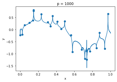
## Results
``` python
ps = list(range(3, 20)) + [30, 50, 100, 150, 200, 300, 400, 500, 1000]
scales = [0.01, 0.1, 1.0]
result = [ evaluate_model(PolynomialWithRandomFeatures(scale=scale), X, y, len(y), ps, runs=100) for scale in scales ]
result = np.array(result)
```
``` python
p = plt.plot(ps, result.T)
[ plt.axvline(x=ps[np.argmin(result[i])], color=p[i].get_color(), alpha=0.5, linestyle='--') for i in range(result.shape[0]) ]
plt.legend(scales)
plt.xscale("log")
plt.xlabel("p")
plt.yscale("log")
#plt.ylim(0.1,10)
plt.ylabel("average mse")
plt.show()
```
------------------------------------------------------------------------
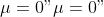
## 4 Legendre polynomial
``` python
class LegendrePolynomialFeatures():
def __call__(self, X, y, n, p, random_state=42):
x = X if len(X.shape) == 1 else X[:,0]
F = np.array([]).reshape(x.shape[0], 0)
# Generate polynomial features
for deg in range(p):
l = np.polynomial.legendre.Legendre([0]*deg + [1], domain=[0,1])
F = np.insert(F, deg, l(x), axis=1)
return F, y
```
------------------------------------------------------------------------
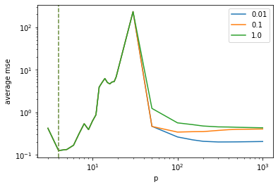
## Demonstration
``` python
F, _ = LegendrePolynomialFeatures()(X, y, len(y), 1000)
g = np.linspace(0, 1, 10000)
G, _ = LegendrePolynomialFeatures()(g, y, len(y), 1000)
```
``` python
clf = MyRidgeRegressor(p=8)
clf.fit(F, y)
plt.plot(g, clf.predict(G))
plt.scatter(X, y)
plt.title("p = 8")
plt.xlabel("x")
plt.ylabel("y")
plt.show()
```
``` python
clf = MyRidgeRegressor(p=50)
clf.fit(F, y)
plt.plot(g, clf.predict(G))
plt.scatter(X, y)
plt.title("p = 100")
plt.xlabel("x")
plt.ylabel("y")
plt.show()
```

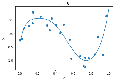
``` python
clf = MyRidgeRegressor(p=1000)
clf.fit(F, y)
plt.plot(g, clf.predict(G))
plt.scatter(X, y)
plt.title("p = 1000")
plt.xlabel("x")
plt.ylabel("y")
plt.show()
```
------------------------------------------------------------------------
## Results
``` python
ps = list(range(3, 20)) + [30, 50, 100, 150, 200, 300, 400, 500, 1000]
result = evaluate_model(LegendrePolynomialFeatures(), X, y, len(y), ps, runs=1)
```
``` python
p = plt.plot(ps, result)
plt.axvline(x=ps[np.argmin(result)], color=p[0].get_color(), alpha=0.5, linestyle='--')
plt.legend(scales)
plt.xscale("log")
plt.xlabel("p")
plt.yscale("log")
plt.ylim(0.1,10)
plt.ylabel("mse")
plt.show()
```

------------------------------------------------------------------------
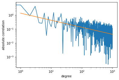
## Correlation analysis
To understand why we are seeing a double descent curve for Legendre
polynomials, we compute the correlation between features
 and response
:
``` python
cor = []
for i in range(F.shape[1]):
cor.append(np.abs(np.correlate(F[:,i], y)))
```
A plot of the result shows that the correlation decreases exponentially,
whereby we are essentially adding noise to the feature matrix
.
``` python
cor_x = np.log(list(range(1, len(cor)+1)))
cor_x = np.array(cor_x).reshape(-1, 1)
cor_y = np.log(cor)
cor_z = np.linspace(1, len(cor), 100).reshape(-1, 1)
clf = LinearRegression()
clf.fit(cor_x, cor_y)
plt.plot(cor)
plt.plot(cor_z, np.exp(clf.predict(np.log(cor_z))))
plt.xscale('log')
plt.xlabel('degree')
plt.yscale('log')
plt.ylabel('absolute correlation')
plt.show()
```
``` python
```