https://github.com/pedroj/bipartite_plots
`ggbipart`, an R package for plotting bipartite networks
https://github.com/pedroj/bipartite_plots
adjacency bipartite-networks ecological-network network-visualization networks networks-biology plotting-bipartite-networks
Last synced: 6 months ago
JSON representation
`ggbipart`, an R package for plotting bipartite networks
- Host: GitHub
- URL: https://github.com/pedroj/bipartite_plots
- Owner: pedroj
- License: gpl-3.0
- Created: 2013-07-09T21:07:57.000Z (about 13 years ago)
- Default Branch: master
- Last Pushed: 2025-04-01T18:43:06.000Z (over 1 year ago)
- Last Synced: 2025-04-01T19:42:57.225Z (over 1 year ago)
- Topics: adjacency, bipartite-networks, ecological-network, network-visualization, networks, networks-biology, plotting-bipartite-networks
- Language: HTML
- Homepage:
- Size: 51.2 MB
- Stars: 32
- Watchers: 7
- Forks: 17
- Open Issues: 1
-
Metadata Files:
- Readme: README.md
- License: LICENSE
Awesome Lists containing this project
README
`ggbipart`: An `R` package for plotting bipartite networks
========================================================
The `ggbipart` package includes a series of `R` functions aimed to plot bipartite networks. Bipartite networks are a special type of network where nodes are of two distinct types or sets, so that connections (links) only exist among nodes of the different sets.
As in other types of network, bipartite structures can be binary (only the presence/absence of the links is mapped) or quantitative (weighted), where the links can have variable importance or weight.
To plot, we start with an adjacency or incidence matrix. I'm using matrices that illustrate ecological interactions among species, such as the mutualistic interactions of animal pollinators and plant flowers. The two sets (modes) of these bipartite networks are animals (pollinators) and plants species.
From any adjacency matrix we can get a `network` object or an `igraph` object for plotting and analysis. The main function in the package is `bip_ggnet`.
### Installation
```r
devtools::install_github("pedroj/bipartite_plots")
library(ggbipart)
```
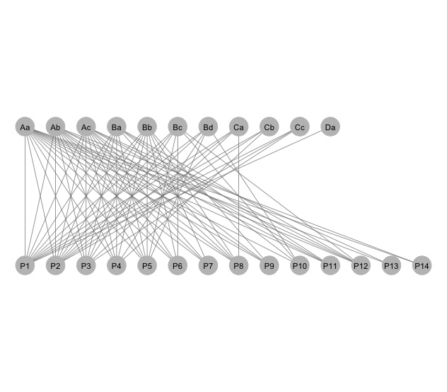
### An unweighted, binary network
This graph uses function `bip_railway`.
```r
# Plot layout coordinates for railway networkplot. Input is the
# adjacency matrix.
#
mymat <- read.delim("./data/data.txt", row.names=1) # Not run.
g<- bip_railway(mymat, label=T)
g+ coord_flip()
```
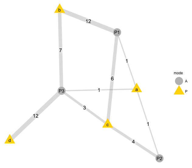
### A weighted network with edges labelled
This graph uses function `bip_ggnet`, with labelled edges.
```r
#-----------------------------------------------------------
# Simple graph prototype for a weighted network.
bip= data.frame(P1= c(1, 12, 6, 0),
P2= c(1, 0, 4, 0),
P3= c(1, 7, 3, 12),
row.names= letters[1:4])
col= c("A"= "grey80", "P"= "gold2")
bip.net<- bip_init_network(as.matrix(bip))
bip_ggnet(bip.net, as.matrix(bip),
# color= "mode", palette = col,
edge.label = "weights",
label= TRUE)
#-----------------------------------------------------------
#
```
### A weighted network with nodes numbered
This graph uses function `bip_ggnet`, with labelling nodes modified with additional `geoms`.
```r
#-----------------------------------------------------------
# Numbered nodes
# The Nava de las Correhuelas dataset.
nch<- read.table("./data/sdw01_adj_fru.csv",
header=T, sep=",", row.names=1,
dec=".", na.strings="NA")
nch.net<- bip_init_network(as.matrix(nch))
nums<- as.vector(c(1:sum(dim(nch))))
pp3<- bip_ggnet(nch.net, as.matrix(nch),
size= 0,
shape= "mode",
palette= "Set1",
color= "mode",
layout.exp = 0.25) +
geom_point(aes(color= color), size= 10,
color= "white") +
geom_point(aes(color= color), size= 10,
alpha= 0.5) +
geom_point(aes(color= color), size= 8) +
geom_text(aes(label= nums),
color= "white", size= 3.5,
fontface="bold") +
guides(color= FALSE) +
theme(legend.position="none") # Hide legend
pp3
#-----------------------------------------------------------
#
```

A detailed descripton of all the above code is in my [git pages](http://pedroj.github.io/bipartite_plots/).
[ ](https://creativecommons.org/licenses/by-nc/4.0/)