https://github.com/precise-simulation/distmesh-julia
DistMesh-Julia - Simple Mesh Generation in Julia
https://github.com/precise-simulation/distmesh-julia
julia matlab mesh mesh-generation mesh-generator octave simulation
Last synced: about 1 year ago
JSON representation
DistMesh-Julia - Simple Mesh Generation in Julia
- Host: GitHub
- URL: https://github.com/precise-simulation/distmesh-julia
- Owner: precise-simulation
- License: other
- Created: 2022-05-09T07:30:18.000Z (about 4 years ago)
- Default Branch: main
- Last Pushed: 2022-05-09T07:35:18.000Z (about 4 years ago)
- Last Synced: 2025-04-01T02:53:01.113Z (over 1 year ago)
- Topics: julia, matlab, mesh, mesh-generation, mesh-generator, octave, simulation
- Language: Julia
- Homepage: https://www.featool.com/grid/2018/03/06/Matlab-Mesh-Generation-Comparison.html
- Size: 36.1 KB
- Stars: 8
- Watchers: 3
- Forks: 1
- Open Issues: 0
-
Metadata Files:
- Readme: README.md
- License: LICENSE
Awesome Lists containing this project
README
DistMesh-Julia - Simple Mesh Generation in Julia
================================================
About DistMesh-Julia
--------------------
DistMesh is a simple Julia code for automatic generation of
unstructured 2D triangular and 3D tetrahedral volume meshes using
(level set) distance functions for describing geometries and domains.
This repository is a Julia port of the consolidated
[2D/3D DistMesh implementation for MATLAB and Octave](https://github.com/precise-simulation/distmesh).
Description
-----------
The original DistMesh MATLAB algorithm was invented by Per-Olof
Persson and Gilbert Strang in the Department of Mathematics at
MIT. More detailed descriptions of the DistMesh algorithm and the
original MATLAB mesh generation code can be found in the SIAM Review
paper and other references linked below.
The simplicity of the DistMesh algorithm is due to using signed
distance functions (level sets) to specify and describe domains,
geometries, and regions to mesh. Distance functions specify the
shortest distance from any point in space to the boundary of the
domain, where the sign of the function is positive outside the region,
negative inside, and zero on the boundary. This definition is used to
identify if a point is located in or outside of the
geometry. Moreover, the gradient of the distance function points in
the direction of the boundary, allowing points outside to be
efficiently moved back to the domain.
A simple example is the unit circle in two dimensions, which has the
distance function _d(r) = r-1_, where _r = sqrt(x^2+y^2)_ is the
distance from the origin. For more complicated geometries the distance
function can be computed by interpolation between values on a grid,
which is a common representation for level set methods.
For the mesh generation procedure, DistMesh uses the Delaunay
triangulation routine in the VornoiDelaunay Julia module and tries to
optimize the node locations by a force-based smoothing procedure. The
topology is regularly updated by Delaunay. The boundary points are
only allowed to move tangentially to the boundary by projections using
the distance function. This iterative procedure typically results in
very uniform and well-shaped high quality meshes.
Usage
-----
To use the this mesh generation code, simply download the stand alone
[distmesh](https://github.com/precise-simulation/distmesh-julia/blob/master/DistMesh.jl)
source code and run it in Julia (tested under Julia v6.2). The
function syntax is as follows
(P, T, STAT) = DISTMESH( FD, FH, H0, BBOX, P_FIX, E_FIX, IT_MAX, FID)
where **FD** is a function handle to the geometry description that
should take evaluation coordinates and points as input. For example
fd = p -> sqrt.(sum(p.^2,2)) - 1 specifies the distance
function for a unit circle (both function handles, string function
names, and anonymous functions are supported). Similar to _FD_, **FH**
a function describing the desired relative mesh size distribution. For
example fh = p -> ones(size(p,1),1) specifies a uniform
distribution where _FH_ evaluates to _1_ at all points. **H0** is a
numeric scalar specifying the initial edge lengths, and **BBOX** is a
2 by 2 in 2D (or 2 by 3 in 3D) bounding box of the domain (enclosing
the zero contour/level set of _FD_). **P_FIX** optionally specifies a
number of points that should always be present (fixed) in the
resulting mesh. **E_FIX** can be sets of edge vertex indices to
constrain, or alternatively a cell array with function handle to call.
**IT_MAX** sets the maximum number of grid generation iterations
allowed (default _1000_). Finally, **FID** specifies a file
identifies for output (default _1_ = terminal output).
The DistMesh-Julia function returns the grid point vertices in **P**,
triangulated simplices in **T**, as well as an optional statistics
struct **STAT** including timings and convergence information.
Input:
FD: Distance function d(x,y,(z))
FH: Scaled edge length function h(x,y,(z))
H0: Initial edge length
BBOX: Bounding box [xmin ymin (zmin); xmax,ymax,(zmax)]
P_FIX: Fixed node positions [N_P_FIX x 2/3]
E_FIX: Constrained edges [N_E_FIX x 2]
IT_MAX: Maximum number of iterations
FID: Output file id number (default 1 = terminal)
Output:
P: Grid vertex/node coordinates [N_P x 2/3]
T: Triangle indices [N_T x 3]
STAT: Mesh generation statistics (struct)
Examples
--------
To automatically run the collection of basic mesh generation examples
described below, type
[distmesh_demo](https://github.com/precise-simulation/distmesh-julia/blob/master/distmesh_demo.jl)
into the Julia command prompt from the directory where the _distmesh_
files can be found.
- Example 1: (Uniform mesh on unit circle)
fd = p -> sqrt.(sum(p.^2,2)) - 1
fh = p -> ones(size(p,1))
(p, t) = distmesh( fd, fh, 0.1, [-1 -1;1 1] )
plotgrid( p, t )
- Example 2: (Uniform mesh on ellipse)
fd = p -> p[:,1].^2/2^2 + p[:,2].^2/1^2 - 1
fh = p -> ones(size(p,1))
(p, t) = distmesh( fd, fh, 0.2, [-2 -1;2 1], [], [], 200 )
plotgrid( p, t )
- Example 3: (Uniform mesh on unit square)
fd = p -> -minimum([minimum([minimum([p[:,2] 1-p[:,2]],2) p[:,1]],2) 1-p[:,1]],2)
fh = p -> ones(size(p,1))
(p, t) = distmesh( fd, fh, 0.2, [-1 -1;1 1], [-1 -1;-1 1;1 -1;1 1] )
plotgrid( p, t )
- Example 4: (Uniform mesh on complex polygon)
pv = [-0.4 -0.5;0.4 -0.2;0.4 -0.7;1.5 -0.4;0.9 0.1;
1.6 0.8;0.5 0.5;0.2 1;0.1 0.4;-0.7 0.7;-0.4 -0.5]
fd = p -> dpolygon( p, pv )
fh = p -> ones(size(p,1))
(p, t) = distmesh( fd, fh, 0.1, [-1 -1;2 1], pv )
plotgrid( p, t )
- Example 5: (Rectangle with circular hole, refined at circle boundary)
fd = p -> maximum( [dpolygon(p,[-1 -1;1 -1;1 1;-1 1;-1 -1]) -(sqrt.(sum(p.^2,2))-0.5)], 2 )
fh = p -> 0.05 + 0.3*(sqrt.(sum(p.^2,2))-0.5)
plotgrid( p, t )
- Example 6: (Square, with size function point and line sources)
dcircle = (p,xc,yc,r) -> sqrt.((p[:,1]-xc).^2+(p[:,2]-yc).^2)-r
fd = p -> -minimum([minimum([minimum([p[:,2] 1-p[:,2]],2) p[:,1]],2) 1-p[:,1]],2)
fh = p -> minimum([minimum(hcat(0.01+0.3*abs.(dcircle(p,0,0,0)),
0.025+0.3*abs.(dpolygon(p,[0.3 0.7;0.7 0.5;0.3 0.7]))),2) 0.15*ones(size(p,1),1)],2)
(p, t) = distmesh( fd, fh, 0.01, [0 0;1 1], [0 0;1 0;0 1;1 1] )
plotgrid( p, t )
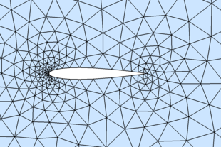
- Example 7: (NACA0012 airfoil)
hlead = 0.01; htrail = 0.04; hmax = 2; circx = 2; circr = 4
a = 0.12/0.2*[0.2969 -0.126 -0.3516 0.2843 -0.1036]
dcircle = (p,xc,yc,r) -> sqrt.((p[:,1]-xc).^2+(p[:,2]-yc).^2)-r
fd = p -> maximum(hcat( dcircle(p,circx,0,circr),
-((abs.(p[:,2])-polyval([a[5:-1:2];0],p[:,1])).^2-a[1]^2*p[:,1]) ), 2 )
fh = p -> minimum([minimum([hlead+0.3*dcircle(p,0,0,0) htrail+0.3*dcircle(p,1,0,0)],2) hmax*ones(size(p,1),1)],2)
fixx = 1 - htrail*cumsum(1.3.^(0:4)')
fixy = a[1]*sqrt.(fixx) + polyval([a[5:-1:2];0],fixx)
pfix = [[circx+[-1 1 0 0]*circr; 0 0 circr*[-1 1]]'; 0 0; 1 0; fixx' fixy'; fixx' -fixy']
bbox = [circx-circr -circr; circx+circr circr]
h0 = minimum([hlead htrail hmax])
(p, t) = distmesh( fd, fh, h0, bbox, pfix )
plotgrid( p, t )
- Example 8: (Uniform mesh on unit sphere)
fd = p -> sqrt.(sum(p.^2,2)) - 1
fh = p -> ones(size(p,1),1)
(p,t) = distmesh( fd, fh, 0.2, [-1 -1 -1;1 1 1] )
plotgrid( p, t )
- Example 9: (Uniform mesh on unit cube)
fd = p -> -minimum([minimum([minimum([minimum([minimum([p[:,3] 1-p[:,3]],2) p[:,2]],2) 1-p[:,2]],2) p[:,1]],2) 1-p[:,1]],2)
fh = p -> ones(size(p,1),1)
pfix = [-1 -1 -1;-1 1 -1;1 -1 -1;1 1 -1; -1 -1 1;-1 1 1;1 -1 1;1 1 1]
(p,t) = distmesh( fd, fh, 0.2, [-1 -1 -1;1 1 1], pfix )
plotgrid( p, t )
- Example 10: (Uniform mesh on cylinder)
fd = p -> -minimum([minimum([p[:,3] 4-p[:,3]],2) 1-sqrt.(sum(p[:,1:2].^2,2))],2)
fh = p -> ones(size(p,1),1)
pfix = [-1 -1 -1;-1 1 -1;1 -1 -1;1 1 -1; -1 -1 1;-1 1 1;1 -1 1;1 1 1]
(p,t) = distmesh( fd, fh, 0.5, [-1 -1 0;1 1 4] )
plotgrid( p, t )
Dependencies
------------
- VornoiDelaunay.jl
- Plots.jl
Issues
------
- 3D is technically supported by DistMesh-Julia, but Julia is missing
a _3D Delaunay_ triangulation functionality.
- Proper module bundling not implemented.
References
----------
[1] [P.-O. Persson, G. Strang, A Simple Mesh Generator in MATLAB. SIAM Review, Volume 46 (2), pp. 329-345, June 2004.](http://persson.berkeley.edu/distmesh/persson04mesh.pdf)
[2] [P.-O. Persson, Mesh Generation for Implicit Geometries. Ph.D. thesis, Department of Mathematics, MIT, Dec 2004.](http://persson.berkeley.edu/thesis/persson-thesis-color.pdf)
[3] [P.-O. Persson's DistMesh website](http://persson.berkeley.edu/distmesh/)
Alternative Implementations
---------------------------
[4] [Consolidated 2D/3D DistMesh for MATLAB and Octave](https://github.com/precise-simulation/distmesh)
[5] [libDistMesh - A Simple Mesh Generator in C++](https://github.com/pgebhardt/libdistmesh)
[6] [PyDistMesh - A Simple Mesh Generator in Python](https://github.com/bfroehle/pydistmesh)
[7] [Mesh generator - Java implementation of DistMesh](https://github.com/plichjan/jDistMesh)
[8] [DistMesh - Wolfram Language Implementation](https://github.com/WolframResearch/DistMesh)
[9] [J. Burkardt's DistMesh repository](http://people.sc.fsu.edu/~jburkardt/m_src/distmesh/distmesh.html)
[10] [KOKO Mesh Generator](http://fc.isima.fr/~jkoko/codes.html)
License
-------
The DistMesh-Julia code is copyrighted by J.S. Hysing and Precise
Simulation Limited and licensed under the GNU GPL License; see the
License and Copyright notice for more information.