https://github.com/ranfysvalle02/bayesian-nn
Unlike traditional neural networks that provide single-point estimates, BNNs embrace a probabilistic approach, delivering not just predictions but confidence intervals—an essential feature for real-world applications like medical diagnostics, autonomous vehicles, and financial forecasting.
https://github.com/ranfysvalle02/bayesian-nn
Last synced: 3 months ago
JSON representation
Unlike traditional neural networks that provide single-point estimates, BNNs embrace a probabilistic approach, delivering not just predictions but confidence intervals—an essential feature for real-world applications like medical diagnostics, autonomous vehicles, and financial forecasting.
- Host: GitHub
- URL: https://github.com/ranfysvalle02/bayesian-nn
- Owner: ranfysvalle02
- Created: 2024-11-11T15:30:06.000Z (11 months ago)
- Default Branch: main
- Last Pushed: 2024-11-17T05:03:03.000Z (11 months ago)
- Last Synced: 2025-06-15T23:06:08.680Z (4 months ago)
- Language: Python
- Homepage:
- Size: 645 KB
- Stars: 0
- Watchers: 1
- Forks: 0
- Open Issues: 0
-
Metadata Files:
- Readme: README.md
Awesome Lists containing this project
README
# bayesian-nn

---
### **Demystifying Bayesian Neural Networks: A Probabilistic Approach to Smarter AI**
In traditional neural networks, when we make a prediction, we get a single output. For example, in a binary classification problem, we might get a single probability that a given input belongs to the positive class.
However, in many real-world scenarios, we want to know more than just the most likely prediction. We want to know how certain the model is about its prediction. This is where Bayesian Neural Networks (BNNs) come in.
A BNN, unlike a traditional neural network, doesn't just output a single prediction. Instead, it outputs a distribution of predictions. This is achieved by using dropout during both training and prediction. During prediction, we run the model multiple times (Monte Carlo sampling), each time with a different dropout mask, and collect all the outputs.
The mean of this distribution is the model's prediction, similar to a traditional neural network. However, the spread of the distribution (often measured by standard deviation or variance) gives us a measure of the model's uncertainty about its prediction.
If the model is very certain, all the predictions will be close to the mean, and the spread will be small. If the model is uncertain, the predictions will be spread out over a larger range, and the spread will be large.
In the quantum world, particles exist in a state of superposition, embodying multiple possibilities at once until observed. Similarly, in the world of BNNs, the model's weights aren't fixed but exist in a state of probabilistic flux, representing a multitude of potential realities.
---
### **Introduction: The Power of Probabilities in AI and Reality**
Artificial intelligence (AI) is reshaping our world, from self-driving cars to natural language processing, and **Bayesian Neural Networks (BNNs)** are at the forefront of making AI smarter, more interpretable, and more reliable. Traditional neural networks have transformed numerous industries, but their inability to model uncertainty leaves them vulnerable to poor decision-making, especially in complex, unpredictable environments.
Bayesian Neural Networks step in to fill this gap. These probabilistic models go beyond deterministic weights and values, embracing uncertainty as a central component of intelligence. But what if I told you that the concept of uncertainty isn’t just fundamental to AI, but to the very nature of reality itself? At the atomic level, particles behave probabilistically, existing in states of superposition, uncertainty, and probability. Waves and particles, once thought to be opposites, merge into a unified whole through quantum mechanics. What if the way AI handles uncertainty echoes the very principles of the universe?
---
### **Bayesian Neural Networks: Where Probability Meets Intelligence**
Let’s start with the basics. Traditional neural networks are trained by adjusting the weights of connections between neurons, with each weight representing the strength of influence between two neurons. Once trained, these weights are fixed, and the network uses them to make predictions. This approach, while effective, fails to account for uncertainty in the real world. What if the data is noisy? What if the model faces unfamiliar situations? Traditional neural networks may struggle to provide reliable predictions when faced with uncertainty.
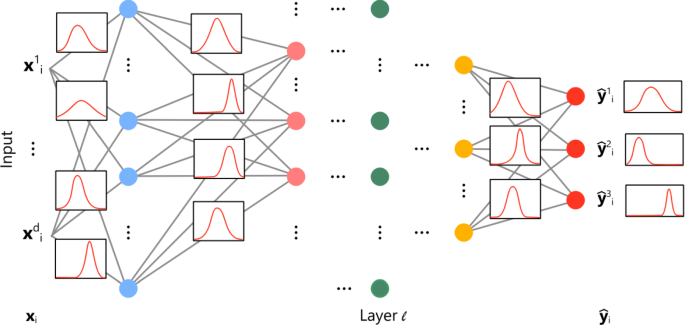
Enter **Bayesian Neural Networks (BNNs)**. Instead of treating the weights as fixed values, BNNs treat the weights as **probability distributions**. This allows the network to represent uncertainty about what the optimal weights might be. In essence, instead of learning a single set of weights, the model learns a distribution over many possible weights, each with varying degrees of confidence. This probabilistic approach allows the model to account for uncertainty in both the data and the environment, leading to more reliable, informed predictions.
In Bayesian terms, we update our belief about the weights as we observe more data, much like how our understanding of the world evolves based on new information. This process is governed by **Bayes' Theorem**, a cornerstone of probability theory:
.png)
Through this probabilistic process, BNNs offer a more holistic way of making predictions — not just an answer, but a **confidence** level, providing insights into how sure (or unsure) the model is about its conclusions.
---
### BNN vs NN
Bayesian Neural Networks (BNNs) differ from traditional neural networks primarily in how they handle uncertainty, but this distinction leads to significant differences in their functionality and applications.
**Key Differences:**
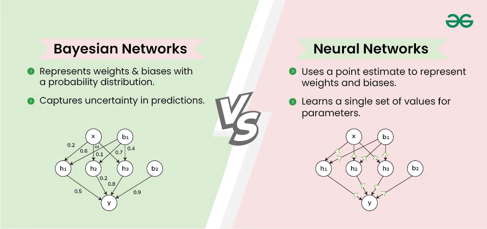
1. **Treatment of Weights:**
- **Traditional Neural Networks (NNs):** The weights are fixed values once the network is trained. The model learns a single optimal set of weights that minimizes the loss function on the training data.
- **Bayesian Neural Networks (BNNs):** The weights are treated as probability distributions rather than fixed values. Instead of finding a single best weight, BNNs infer a distribution over possible weights, capturing the uncertainty about which weights are most appropriate.
2. **Uncertainty Quantification:**
- **Traditional NNs:** Provide point estimates in their outputs without a measure of confidence or uncertainty. They might output a probability in classification tasks, but this is not a true measure of the model's confidence.
- **BNNs:** Offer a principled way to quantify uncertainty in predictions. They output a distribution over possible outputs, allowing you to assess the confidence or uncertainty associated with each prediction.
3. **Inference Process:**
- **Traditional NNs:** Use deterministic optimization methods like gradient descent to find the weights that minimize the loss function.
- **BNNs:** Use Bayesian inference to update the probability distributions of the weights based on the observed data. This often involves approximations like variational inference or Monte Carlo methods due to computational complexity.
4. **Overfitting and Generalization:**
- **Traditional NNs:** Can overfit the training data, especially with limited data or complex models.
- **BNNs:** The probabilistic framework provides a form of regularization, potentially reducing overfitting by integrating over many possible models.
5. **Computational Complexity:**
- **Traditional NNs:** Generally faster to train and easier to implement.
- **BNNs:** More computationally intensive due to the need to approximate the posterior distributions over weights.
**Implications of Uncertainty Modeling:**
- **Decision-Making Under Uncertainty:** In critical applications (e.g., medical diagnosis, autonomous vehicles), knowing the confidence level of predictions is crucial. BNNs provide this information, whereas traditional NNs do not.
- **Active Learning and Exploration:** BNNs can identify instances where the model is uncertain and might benefit from additional data, guiding data collection efforts.
- **Robustness to Overfitting:** By considering a distribution over weights, BNNs can generalize better to unseen data compared to traditional NNs that may overfit.
**Is It Just the Uncertainty Part?**
While uncertainty modeling is the primary difference, it has far-reaching effects:
- **Model Interpretability:** BNNs allow practitioners to understand and interpret the model's confidence, making it more transparent.
- **Risk Assessment:** In applications where incorrect predictions have high costs, knowing the uncertainty helps in risk management.
- **Adaptive Learning:** BNNs can naturally update their beliefs as new data comes in, making them suitable for non-stationary environments.
So, while both traditional neural networks and Bayesian Neural Networks aim to learn from data and make predictions, BNNs extend traditional NNs by incorporating uncertainty directly into the model. This is more than just an added feature; it fundamentally changes how the model learns from data, makes predictions, and can be applied in real-world scenarios where understanding uncertainty is essential.
---
### **Understanding Bayesian Inference in Neural Networks**
Bayesian inference is a method of statistical inference that updates the probability for a hypothesis as more evidence or information becomes available. In the context of neural networks, Bayesian inference is used to estimate the distribution of weights.
In a traditional neural network, the weights are learned through optimization techniques like gradient descent, and they are fixed after training. However, in a Bayesian Neural Network (BNN), the weights are considered as random variables. The goal is not to find the best single set of weights, but rather to determine the distribution of weights that best explain the data.
This is achieved through Bayes' theorem, which in the context of neural networks can be expressed as:
P(weights | data) = [ P(data | weights) * P(weights) ] / P(data)
Here:
- P(weights | data) is the **posterior** distribution of the weights given the data. This is what we want to compute.
- P(data | weights) is the **likelihood** of the data given the weights. This is computed based on the network's architecture and the activation function.
- P(weights) is the **prior** distribution of the weights. This represents our belief about the weights before seeing the data.
- P(data) is the **evidence** or marginal likelihood of the data. This is often difficult to compute directly, so we usually use techniques like Markov Chain Monte Carlo (MCMC) or Variational Inference to approximate the posterior distribution.
The result is a distribution of weights instead of a single set. This allows the BNN to capture the uncertainty in the weights, which in turn provides a measure of uncertainty in the predictions.
---
### **Quantifying Uncertainty in Bayesian Neural Networks**
One of the key advantages of Bayesian Neural Networks is their ability to quantify uncertainty. This is achieved through the distribution of weights and the use of dropout during prediction.
In a BNN, dropout is not only used during training but also during prediction. This is known as Monte Carlo Dropout. During prediction, we run the model multiple times, each time with a different dropout mask, and collect all the outputs. This gives us a distribution of predictions for each input.
The mean of this distribution is the model's prediction, similar to a traditional neural network. However, the spread of the distribution (often measured by standard deviation or variance) gives us a measure of the model's uncertainty about its prediction.
If the model is very certain, all the predictions will be close to the mean, and the spread will be small. If the model is uncertain, the predictions will be spread out over a larger range, and the spread will be large.
---
### **Building a Bayesian Neural Network for Sentiment Analysis with Feedback Integration**
---
### 1. Understanding Bayesian Neural Networks
Bayesian Neural Networks introduce uncertainty estimates into deep learning models by integrating Bayesian inference. Unlike traditional neural networks, BNNs provide probability distributions over the weights and outputs, allowing the model to express uncertainty about its predictions.
**Advantages:**
- **Uncertainty Estimation:** Provides confidence intervals for predictions.
- **Robustness:** Better generalization to unseen data.
- **Adaptive Learning:** Capable of updating beliefs with new data.
### 2. Loading Pre-trained Word Embeddings
We use GloVe (Global Vectors for Word Representation) embeddings to convert words into numerical vectors that capture semantic meaning.
```python
def load_glove_embeddings(glove_file_path='glove.6B.300d.txt'):
embeddings = {}
with open(glove_file_path, 'r', encoding='utf-8') as f:
for line in f:
values = line.strip().split()
word = values[0]
vector = torch.tensor([float(val) for val in values[1:]], dtype=torch.float32)
embeddings[word] = vector
return embeddings
```
**Note:** Ensure you have the `glove.6B.300d.txt` file in your working directory.
### 3. Creating a Synthetic Sentiment Dataset
To simulate a realistic environment, we create a synthetic dataset with predefined positive and negative sentences.
```python
class SentimentDataset(Dataset):
def __init__(self, num_samples=1000, embeddings=None):
self.embeddings = embeddings if embeddings else {}
self.positive_sentences = [
"I love this product!",
"Absolutely fantastic experience.",
# ... more positive sentences ...
]
self.negative_sentences = [
"This is terrible.",
"Absolutely horrible experience.",
# ... more negative sentences ...
]
self.texts = []
self.labels = []
for i in range(num_samples):
if i % 2 == 0:
sentence = random.choice(self.positive_sentences)
label = 1
else:
sentence = random.choice(self.negative_sentences)
label = 0
self.texts.append(sentence)
self.labels.append(label)
```
**Tokenization and Embedding:**
We clean, tokenize, and convert each sentence into a fixed-length embedding vector using GloVe embeddings.
### 4. Building the Data Module
Using PyTorch Lightning's `LightningDataModule`, we handle data preparation, including training-validation split and data loading.
```python
class SentimentDataModule(pl.LightningDataModule):
def __init__(self, batch_size=BATCH_SIZE, num_samples=NUM_SAMPLES, embeddings=None):
super().__init__()
self.batch_size = batch_size
self.num_samples = num_samples
self.embeddings = embeddings
self.train_dataset = None
self.val_dataset = None
def setup(self, stage=None):
if self.train_dataset is not None and self.val_dataset is not None:
return
dataset = SentimentDataset(num_samples=self.num_samples, embeddings=self.embeddings)
train_size = int(0.8 * len(dataset))
val_size = len(dataset) - train_size
self.train_dataset, self.val_dataset = random_split(dataset, [train_size, val_size])
```
**Incorporating Feedback Data:**
We add a method `add_feedback` to include new feedback data into the training dataset.
```python
def add_feedback(self, feedback_texts, feedback_labels):
# Tokenize and create a TensorDataset for feedback
# Concatenate with the existing training dataset
self.train_dataset = ConcatDataset([self.train_dataset, feedback_tensor_dataset])
```
### 5. Defining the Bayesian Neural Network Model
We construct the BNN using Monte Carlo Dropout layers to approximate Bayesian inference.
```python
class BayesianNN(pl.LightningModule):
def __init__(self, input_dim=INPUT_DIM, hidden_dim=HIDDEN_DIM, output_dim=OUTPUT_DIM, p=DROPOUT_PROB, lr=LEARNING_RATE):
super(BayesianNN, self).__init__()
self.save_hyperparameters()
self.fc1 = nn.Linear(input_dim, hidden_dim)
self.dropout1 = nn.Dropout(p)
self.fc2 = nn.Linear(hidden_dim, hidden_dim)
self.dropout2 = nn.Dropout(p)
self.fc3 = nn.Linear(hidden_dim, output_dim)
self.activation = nn.ReLU()
self.loss_fn = nn.BCEWithLogitsLoss()
def forward(self, x):
x = self.activation(self.fc1(x))
x = self.dropout1(x)
x = self.activation(self.fc2(x))
x = self.dropout2(x)
x = self.fc3(x)
return x
```
**Predicting with Uncertainty:**
We perform multiple forward passes with dropout enabled to estimate uncertainty.
```python
def predict_sentiment(self, x, num_samples=MC_SAMPLES):
self.train()
predictions = []
with torch.no_grad():
for _ in range(num_samples):
logits = self(x)
preds = torch.sigmoid(logits)
predictions.append(preds)
predictions = torch.stack(predictions)
mean_prediction = torch.mean(predictions, dim=0)
uncertainty = torch.std(predictions, dim=0)
self.eval()
return mean_prediction, uncertainty
```
### 6. Training the Model
We initialize and train the model using PyTorch Lightning's `Trainer`.
```python
model = BayesianNN()
trainer = pl.Trainer(
max_epochs=EPOCHS,
callbacks=[progress_bar, early_stop_callback, lr_monitor],
deterministic=True
)
trainer.fit(model, datamodule=data_module)
```
### 7. Making Predictions Before Feedback
Before incorporating feedback, we test the model on a set of sample texts.
**Sample Predictions:**
```
Text: "This product is amazing!"
Prediction: 0.0244 (Negative)
Uncertainty: 0.0991
Text: "I hate this item."
Prediction: 0.6569 (Positive)
Uncertainty: 0.3535
```
**Observations:**
- The model incorrectly predicts some sentiments.
- High uncertainty indicates the model's lack of confidence.
### 8. Incorporating User Feedback
We gather user feedback to improve the model's predictions.
```python
feedback_texts = [
"This product is amazing!",
"Absolutely love it!",
# ... more feedback texts ...
]
feedback_labels = [1]*10 + [0]*10 # 10 positive and 10 negative
data_module.add_feedback(feedback_texts, feedback_labels)
```
**Process:**
- **Collect Feedback:** Gather new data points with correct labels.
- **Add to Dataset:** Incorporate the feedback into the training data.
- **Retrain the Model:** Update the model with the new data.
### 9. Retraining the Model with Feedback
We retrain the model using the updated dataset.
```python
# Reinitialize the trainer to reset optimizer states
trainer = pl.Trainer(
max_epochs=EPOCHS,
callbacks=[progress_bar, early_stop_callback, lr_monitor],
deterministic=True
)
trainer.fit(model, datamodule=data_module)
```
**Ensuring Training Mode:**
Before retraining, set the model back to training mode to enable parameter updates.
```python
model.train()
```
### 10. Observing the Improvements
After retraining, we make predictions on the same sample texts.
**Updated Predictions:**
```
Text: "This product is amazing!"
Prediction: 0.9986 (Positive)
Uncertainty: 0.0134
Text: "I hate this item."
Prediction: 0.0000 (Negative)
Uncertainty: 0.0003
```
**Improvements:**
- The model now correctly predicts sentiments.
- Reduced uncertainty reflects increased confidence due to new data.
By integrating user feedback, we've enhanced the model's performance significantly. This approach demonstrates the power of Bayesian Neural Networks combined with active learning strategies in creating adaptable NLP models.
**Key Takeaways:**
- **Dynamic Learning:** Models can be updated with new data to improve over time.
- **Uncertainty Estimation:** BNNs provide valuable insights into prediction confidence.
- **User Feedback Integration:** Actively incorporating feedback leads to more accurate and robust models.
---
### **Conclusion: The Infinite Potential of Embracing Uncertainty**
"When nothing is certain, everything is possible." This quote captures the essence of both quantum mechanics and **Bayesian Neural Networks**. We have the opportunity to explore an infinite number of possibilities, learning and evolving as we go. By embracing uncertainty, we can open ourselves to new ways of understanding the world, approaching AI, and engaging with the mysteries of the cosmos.
**Bayesian Neural Networks** offer a unique lens through which we can view the world — one that not only handles uncertainty but thrives in it. Like quantum systems, **BNNs** don’t collapse into a single answer but exist in a state of fluid possibility (in the form of a distribution of weights or outputs). This approach allows us to understand the world not in terms of fixed, deterministic truths, but as a web of interconnected probabilities, each influencing the others. By embracing this view, we not only build smarter AI but also gain a deeper understanding of the universe itself — one that is alive with potential and full of possibilities waiting to be discovered.
---
### When to use BNNs
Bayesian Neural Networks (BNNs) are particularly useful in applications where uncertainty quantification is crucial. Here are some real-world use cases:
1. **Medical Diagnostics**: In healthcare, BNNs can be used to predict the likelihood of a disease given a set of symptoms or test results. The uncertainty quantification can help doctors understand the confidence level of the diagnosis and decide whether further tests are needed.
2. **Autonomous Vehicles**: BNNs can be used in the decision-making process of self-driving cars. For instance, predicting the trajectory of surrounding vehicles or pedestrians. The uncertainty measure can help the system understand the reliability of its predictions and make safer decisions.
3. **Financial Forecasting**: In finance, BNNs can be used to predict stock prices or market trends. The uncertainty measure can help investors understand the risk associated with their investments.
4. **Natural Disaster Prediction**: BNNs can be used to predict the likelihood of natural disasters like earthquakes or floods. The uncertainty measure can help in understanding the confidence level of these predictions and aid in disaster management planning.
5. **Personalized Recommendations**: In recommendation systems, BNNs can be used to predict user preferences with an associated uncertainty. This can help in providing more reliable and personalized recommendations.
---
# Demystifying Hyperparameters in Bayesian Neural Networks

Building a Bayesian Neural Network (BNN) can feel like venturing into uncharted waters. You tweak hyperparameters like epochs and learning rates, but sometimes the model improves without a clear understanding of why. If you've ever wondered why certain hyperparameters work better or worse in a BNN—and found yourself puzzled—you're not alone.
**What Are Bayesian Neural Networks?**
Before diving into hyperparameters, let's briefly revisit what makes BNNs unique. Unlike traditional neural networks that produce point estimates, BNNs provide probability distributions as outputs. This means they can quantify uncertainty in their predictions, making them valuable in fields where understanding confidence levels is crucial.
**The Role of Hyperparameters**
Hyperparameters are the settings that govern the training process of a neural network. They include:
- **Epochs**: The number of times the training algorithm will work through the entire training dataset.
- **Learning Rate**: Determines the step size at each iteration while moving toward a minimum of a loss function.
- **Batch Size**: The number of training examples utilized in one iteration.
In BNNs, these hyperparameters play a significant role in how the model learns the underlying probability distributions.
**Challenges of BNNs Compared to Traditional Neural Networks**
In the provided code, the loss function used is `nn.BCEWithLogitsLoss()`. This is a more complex loss function compared to something like Mean Squared Error (MSE) often used in traditional neural networks.
`nn.BCEWithLogitsLoss()` combines a `Sigmoid` layer and the `BCELoss` (Binary Cross Entropy Loss) in one single class. This version is more numerically stable than using a plain `Sigmoid` followed by a `BCELoss` as, by combining the operations into one layer, we take advantage of the log-sum-exp trick for numerical stability.
The `BCEWithLogitsLoss` computes the loss between the target and the output logits from the network. This is suitable for binary classification problems like the sentiment analysis problem in the provided code. The output of the network is expected to be the raw, unnormalized scores for each class, also known as logits.
In the context of Bayesian Neural Networks (BNNs), the complexity arises from the fact that we are not just optimizing fixed parameters, but we are learning a distribution of parameters. This involves a more complex process of updating beliefs about the parameters as more data is observed, which is inherently a more complex optimization problem.
1. **Complexity of the Loss Function**: BNNs often use more complex loss functions that involve probabilistic components, making optimization trickier.
2. **Computational Overhead**: Sampling from distributions adds computational complexity, leading to longer training times.
3. **Stochasticity**: The inherent randomness in BNNs can make the training process less predictable.
Stochasticity refers to the inherent randomness in the training process. In BNNs, this randomness comes from two main sources:
1. **Random Weight Initialization**: Weights in neural networks are often initialized randomly, which affects the starting point of the optimization process. This is also true for BNNs.
2. **Dropout during Training and Prediction**: In the provided code, dropout is used during both training and prediction (inference). Dropout randomly sets a fraction of input units to 0 at each update during training time, which helps prevent overfitting. This is a form of model complexity control. During prediction, dropout is used to obtain a Monte Carlo approximation of the predictive distribution, introducing additional randomness.
This inherent randomness means that even with the same hyperparameters, two training runs can yield different results. This is why BNNs are often seen as less predictable compared to traditional deterministic neural networks. However, this stochasticity also allows BNNs to capture and quantify uncertainty, which is a key advantage of Bayesian methods.
**Understanding Stochasticity in BNNs**
Stochasticity refers to the randomness inherent in the training process. In BNNs, this comes from:
- **Random Weight Initialization**: Weights are often initialized randomly, affecting the starting point of optimization.
- **Sampling Processes**: BNNs sample from probability distributions during training, introducing variability.
This randomness means that even with the same hyperparameters, two training runs can yield different results.
**Optimization and Convergence**
Optimization algorithms aim to minimize the loss function. Common algorithms include Gradient Descent and its variants like Adam or RMSprop. In BNNs:
- **Gradient Descent**: Helps find the minimum of a function by iteratively moving in the direction of the steepest descent.
- **Convergence**: Reaching a point where further training doesn't significantly change the model's performance.
Because of stochasticity, convergence in BNNs can be less straightforward than in traditional neural networks.
**Tuning Hyperparameters**
Given these challenges, hyperparameter tuning becomes both more critical and more complex.
1. **Epochs**: More epochs allow the model to learn better but can lead to overfitting.
2. **Learning Rate**: A smaller learning rate means smaller steps towards the minimum, which can be good for precision but slow down training.
3. **Batch Size**: Smaller batches introduce more noise but can help the model generalize better.
**Practical Tips for Hyperparameter Tuning**
- **Start Simple**: Begin with standard values (e.g., learning rate of 0.01, batch size of 32) and adjust based on performance.
- **Monitor Training**: Keep an eye on training and validation loss to detect overfitting or underfitting.
- **Use Validation Sets**: Separate data to validate the model's performance during training.
- **Experiment Systematically**: Change one hyperparameter at a time to understand its impact.
**Illustrative Example: Gradient Descent in BNNs**
Imagine you're trying to find the lowest point in a hilly landscape (the minimum of the loss function). Gradient Descent helps you decide which direction to move based on the slope. In BNNs, the landscape is foggy (due to stochasticity), so each step is less certain. Adjusting the learning rate (step size) and epochs (number of steps) can help you navigate this uncertain terrain more effectively.
Navigating the stochastic seas of Bayesian Neural Networks can be challenging, especially when hyperparameters seem to affect the model in unpredictable ways. Understanding the role of hyperparameters and the inherent randomness in BNNs is the first step toward mastering them. As you build intuition through experimentation and observation, you'll find that these once-mysterious settings become valuable tools in your machine learning toolkit.
---
### **Inferential Statistics vs. Bayesian Statistics: A Shift in Perspective**
In the realm of statistics, two major approaches have been widely adopted: **Inferential Statistics** and **Bayesian Statistics**. While both methods aim to understand and interpret data, they differ significantly in their philosophical underpinnings and methodologies.
#### **Inferential Statistics: The Classical Approach**
Inferential Statistics, also known as frequentist statistics, is the traditional approach to statistical analysis. It involves making inferences about populations using data drawn from the population. The key idea is to develop estimates and test hypotheses based on sample data without making assumptions about the underlying population distribution.
Inferential statistics rely heavily on the concept of probability. However, this probability is interpreted as a long-run frequency. For example, if we say there's a 95% confidence interval for a parameter, it means that if we were to repeat the experiment many times, 95% of the intervals would contain the true parameter.
This approach has been the backbone of statistical analysis for many years, providing the foundation for hypothesis testing, confidence intervals, and other statistical procedures. However, it has its limitations, particularly when it comes to handling uncertainty and prior knowledge.
#### **Bayesian Statistics: Embracing Uncertainty**
Bayesian Statistics, on the other hand, provides a mathematical framework for updating beliefs based on data. It is named after Thomas Bayes, who provided the first mathematical treatment of a non-trivial problem of statistical data analysis using what is now known as Bayesian inference.
Unlike inferential statistics, Bayesian statistics interprets probability as a degree of belief or subjective probability. This means that probability can be assigned to any statement, not just repeatable events. Bayesian methods allow for the incorporation of prior knowledge or beliefs into the statistical analysis through the use of a prior probability distribution. As more data is observed, these beliefs are updated using Bayes' theorem.
With the advent of powerful computing resources, Bayesian methods have become increasingly popular. They allow for a more flexible and nuanced approach to statistical analysis, particularly in complex modeling scenarios. Bayesian methods can handle uncertainty more naturally and can incorporate prior knowledge effectively, making them a powerful tool in the modern data scientist's toolkit.
#### **From Inferential to Bayesian: A Paradigm Shift**
The shift from inferential statistics to Bayesian statistics represents a significant paradigm shift. While inferential statistics focus on frequency-based probability and fixed parameters, Bayesian statistics embrace uncertainty and variability. Bayesian methods, in a sense, can be seen as a form of "brute-forcing" towards the convergence of a solution, leveraging computational power to explore the entire parameter space.
This shift has been facilitated by the increased availability of significant computing power, which has made it feasible to perform the complex calculations required for Bayesian methods. As a result, Bayesian methods have found applications in a wide range of fields, from machine learning and artificial intelligence to social sciences and medicine.
---
### **Appendix: Additional Thought-Provoking Concepts**


---
#### **1. The Heisenberg Uncertainty Principle: Embracing the Quantum Unknown**
In a world driven by data and predictability, uncertainty is often seen as something to minimize or eliminate. The goal in traditional machine learning models is to optimize and reduce the error, ensuring that the model provides the most confident, deterministic predictions. However, in the context of **Bayesian Neural Networks**, uncertainty isn't something to fear, but something to **embrace**. When we acknowledge uncertainty, we open ourselves up to more informed, nuanced decision-making.
In quantum mechanics, **uncertainty** is intrinsic — particles do not behave according to fixed rules. This is encapsulated in the **Heisenberg Uncertainty Principle**, which states that the position and momentum of a particle cannot both be precisely measured at the same time. Rather, their behavior is probabilistic. Electrons exist in **superposition**, a state where they occupy multiple possibilities at once, only collapsing into a single state when observed. This is not a flaw but an inherent feature of the quantum world. In much the same way, **Bayesian Neural Networks** understand that data doesn’t provide absolute answers but rather points toward a **distribution of possibilities**. Embracing uncertainty allows for better predictions, especially in complex, unpredictable environments.
This acceptance of uncertainty is a powerful lesson. In both science and life, when we stop clinging to certainty, we create space for growth, exploration, and discovery. It’s in the unknown that we often make our greatest breakthroughs — not just in AI, but in our understanding of the universe itself.
---
#### **2. Existence as a Superposition of Possibilities: The Quantum Analogy**
Imagine a universe in which every possibility exists simultaneously until it is observed. In quantum mechanics, this is the nature of **superposition**. A quantum system, like an electron, doesn’t have a single, fixed state. Instead, it exists in multiple potential states, each with a certain probability, and only "chooses" one when it is measured or observed. This phenomenon, a cornerstone of the Heisenberg Uncertainty Principle, implies that reality itself is not one fixed thing but a web of interconnected possibilities.
Similarly, **Bayesian Neural Networks** operate in a state of superposition. Instead of producing a single, deterministic answer, **BNNs** maintain a distribution of possible outcomes. This distribution represents all the potential scenarios that could unfold given the current data, along with the uncertainty that surrounds each one. The more data the network receives, the more its predictions collapse into a single, more reliable outcome, akin to how the quantum system collapses into a definite state once observed.
This concept of **existence as a superposition of possibilities** invites a new way of thinking about our reality and the AI models that interact with it. What if we stopped thinking about outcomes as fixed points? What if, instead of striving for certainty, we embraced the inherent fluidity of reality — a reality where multiple possibilities exist simultaneously, each with its own likelihood of becoming the "truth"?
In AI, this perspective is incredibly valuable. When we acknowledge the superposition of possibilities, we open the door to more flexible, adaptable systems that are capable of handling uncertainty and complexity in a way traditional deterministic models cannot. This mindset change allows us to approach challenges from a place of openness, where multiple possibilities are always on the table.