https://github.com/ranfysvalle02/explainable-ml
This project provides a comprehensive guide to sentiment analysis using machine learning. It covers the process of turning text into numerical features, building a sentiment analysis model, and enhancing model reliability with explainability using SHAP.
https://github.com/ranfysvalle02/explainable-ml
Last synced: 6 months ago
JSON representation
This project provides a comprehensive guide to sentiment analysis using machine learning. It covers the process of turning text into numerical features, building a sentiment analysis model, and enhancing model reliability with explainability using SHAP.
- Host: GitHub
- URL: https://github.com/ranfysvalle02/explainable-ml
- Owner: ranfysvalle02
- Created: 2024-11-03T14:54:47.000Z (11 months ago)
- Default Branch: main
- Last Pushed: 2024-11-03T17:41:10.000Z (11 months ago)
- Last Synced: 2025-04-12T21:44:36.969Z (6 months ago)
- Language: Python
- Homepage:
- Size: 96.7 KB
- Stars: 0
- Watchers: 1
- Forks: 0
- Open Issues: 0
-
Metadata Files:
- Readme: README.md
Awesome Lists containing this project
README
# explainable-ml

---
# Enhancing Machine Learning with Explainability
Whether it's analyzing customer reviews, gauging public sentiment on social media, or monitoring brand reputation, **sentiment analysis** plays a pivotal role. But how do machines understand and interpret human emotions? Moreover, how can we ensure that these interpretations are transparent and trustworthy? In this blog post, we'll explore the fundamentals of sentiment analysis using classic machine learning techniques, delve into feature extraction, and uncover the importance of explainability in building reliable models.
---
## What is Sentiment Analysis?
Sentiment analysis is a branch of **natural language processing (NLP)** used to determine whether text data expresses positive, negative, or neutral sentiments. For example:
- A movie review: "I absolutely loved this movie!" (Positive)
- A customer review: "The product didn’t meet my expectations." (Negative)
Businesses use sentiment analysis to understand customer feedback, public sentiment, and even brand perception on social media.
---
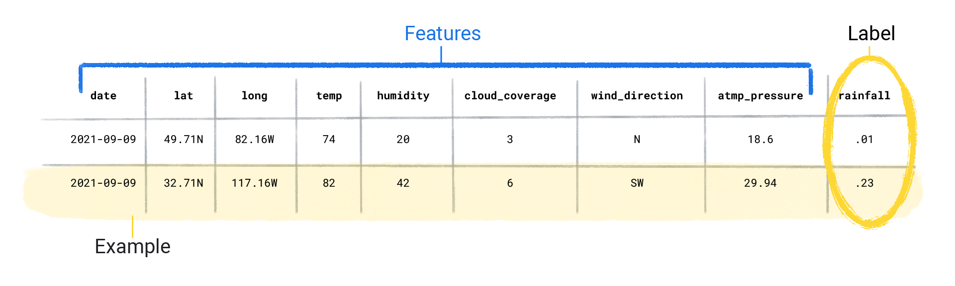
## Step 1: Turning Text into Features
For machine learning algorithms to work with text, we need to **convert words into numerical features**. There are a few common techniques to achieve this transformation, each with unique strengths.
### Tokenization: The First Step in Text Processing
**Tokenization** is the process of breaking down text into smaller components called **tokens**. Tokens can be words, sentences, or phrases, depending on the level of detail we need.
- **Example Sentence:** "I loved this movie."
- **Tokens:** ["I", "loved", "this", "movie"]
Tokenization allows us to isolate each meaningful component of the text, preparing it for further processing.
### [Bag of Words (BoW): Simple Word Counts](https://github.com/ranfysvalle02/just-a-bag-of-words)
The **Bag of Words (BoW)** model is one of the simplest methods for text representation. It captures the presence (or frequency) of each word in a document without regard for word order or grammar.
#### How BoW Works
1. **Tokenize** the text into words.
2. **Count** the occurrences of each unique word across all documents.
3. Represent each document as a **vector** of word counts.
BoW treats each word independently, which is both a strength (simplicity) and a limitation (no understanding of context).
*Example:*
For two reviews:
1. "I love this movie"
2. "This movie is terrible"
A Bag of Words vector would look like this:
| Word | Document 1 | Document 2 |
|--------|------------|------------|
| I | 1 | 0 |
| love | 1 | 0 |
| this | 1 | 1 |
| movie | 1 | 1 |
| is | 0 | 1 |
| terrible | 0 | 1 |
### TF-IDF: Enhancing Feature Significance
**Term Frequency-Inverse Document Frequency (TF-IDF)** is an extension of Bag of Words that weighs each word according to its importance.
- **Term Frequency (TF):** How often a word appears in a document.
- **Inverse Document Frequency (IDF):** How unique a word is across all documents.
The goal of TF-IDF is to highlight words that are frequent in a single document but not common across all documents, providing a more refined feature set. Words that are too common (like "the" or "is") are down-weighted, while unique words that might carry more meaning (like "exceptional" or "dull") are given more weight.
### N-grams: Adding Context
While Bag of Words and TF-IDF focus on individual words, **n-grams** allow us to consider sequences of words to capture more context.
- **Unigram:** A single word, e.g., "movie."
- **Bigram:** A pair of consecutive words, e.g., "good movie."
- **Trigram:** A sequence of three words, e.g., "really good movie."
N-grams can improve a model's understanding by capturing phrases that carry meaning in combination, such as "not bad" (which has a different sentiment than either word alone).
### Vectorization: Converting Words to Numbers
Once we extract tokens, assign weights, or create n-grams, we need to convert them into a numerical representation called **vectorization**. Vectorization represents each document as a **vector** of numbers, allowing machine learning algorithms to process and interpret the text.
---
## Step 2: Building a Sentiment Analysis Model
With features extracted, we can now build a machine learning model. We use **Logistic Regression**, a simple but effective algorithm for binary classification (positive vs. negative). Our steps:
1. **Split the Data:** Reserve some data for testing to evaluate performance on unseen text.
2. **Train the Model:** Use the training data to teach the model which words or phrases are associated with positive and negative sentiments.
3. **Evaluate the Model:** Measure how accurately the model predicts sentiment on the test set.
### Sample Evaluation Metrics
We assess the model with several metrics:
- **Accuracy:** Measures how often the model correctly predicts the sentiment.
- **Confusion Matrix:** Shows true positives, true negatives, false positives, and false negatives.
- **Classification Report:** Breaks down the model’s precision, recall, and F1-score for each class (positive and negative).
*Sample Output:*
```
Model Accuracy: 90.00%
Confusion Matrix:
[[4 1]
[0 5]]
Classification Report:
precision recall f1-score support
Negative 1.00 0.80 0.89 5
Positive 0.83 1.00 0.91 5
```
In this example, the model achieved **90% accuracy**, indicating that it performs well in predicting the sentiment of movie reviews.
---
## Step 3: Explainability – Building Trust with SHAP
High accuracy is great, but understanding **why** a model makes certain predictions is equally important. **Explainability** allows us to interpret model decisions and identify influential features.
### Introducing SHAP (SHapley Additive exPlanations)
**SHAP** is an explainability tool that assigns each feature an importance value for a specific prediction. It provides:
- **Global explanations**: Identifies the most important words across all predictions.
- **Local explanations**: Shows which words influenced an individual prediction.
#### Why Explainability Matters
1. **Trustworthiness:** Helps users understand why a prediction was made.
2. **Debugging:** Reveals patterns or biases, allowing improvements.
3. **Compliance:** Important for models in regulated industries (finance, healthcare) where transparency is required.
### Exploring SHAP in Our Model
*Global Feature Importance:*
```
Top 10 Features Contributing to the Model (Global Importance):
movie: 0.0234
disappointing: 0.0182
lackluster: 0.0160
performances: 0.0128
story: 0.0110
absolutely: 0.0106
plot: 0.0103
failed: 0.0092
uninspired: 0.0083
stunning: 0.0065
```
*Local Feature Explanation for a Single Review:*
For one movie review, SHAP explains which words contributed most to its prediction.
```
Review Text: "I absolutely loved this movie! The performances were stellar and the story was gripping."
Actual Label: Positive
Predicted Label: Positive
Top Contributing Words:
movie: 0.0196 (Positive)
performances: 0.0270 (Positive)
gripping: 0.0154 (Positive)
```
This detailed breakdown shows that **"movie," "performances,"** and **"gripping"** contributed positively to the prediction, aligning with the overall sentiment of the review.
---
## Conclusion: Building Reliable and Explainable Sentiment Models
Sentiment analysis opens a window into understanding opinions and emotions in text, but effective analysis requires a deep understanding of the fundamentals.
**Key Takeaways:**
- **Feature Extraction:** Techniques like **Bag of Words**, **TF-IDF**, **n-grams**, and **vectorization** help convert text into numerical features that models can interpret.
- **Model Evaluation:** Metrics such as accuracy and the confusion matrix are essential to assess a model’s reliability.
- **Explainability with SHAP:** Transparency is crucial for trust and accountability. SHAP allows us to understand why a model makes specific predictions, increasing its trustworthiness.
---
This approach to sentiment analysis serves as a foundation for more advanced methods in NLP. By understanding and utilizing these core principles, we not only improve model performance but also build models that are both effective and transparent. Whether you're analyzing customer feedback, gauging social sentiment, or exploring product reviews, mastering these fundamentals is a powerful step toward creating meaningful and reliable machine learning solutions.
---
# APPENDIX
## Understanding the Confusion Matrix: Measuring Model Performance
After building and training a sentiment analysis model, it's essential to evaluate its accuracy and understand how well it distinguishes between positive and negative sentiments. One of the most informative tools for this is the **Confusion Matrix**.
### What is a Confusion Matrix?
A **Confusion Matrix** is a table used to evaluate the performance of a classification model by comparing the actual vs. predicted outcomes. It provides a breakdown of the model’s predictions, showing where it performs well and where it makes mistakes.
For a binary classification model like our sentiment analysis example, the confusion matrix has four key components:
| | Predicted Positive | Predicted Negative |
|---------------|--------------------|--------------------|
| **Actual Positive** | True Positive (TP) | False Negative (FN) |
| **Actual Negative** | False Positive (FP) | True Negative (TN) |
### Breaking Down the Components
1. **True Positives (TP):** These are cases where the model correctly predicts a positive sentiment for a review that is actually positive.
2. **True Negatives (TN):** These are cases where the model correctly predicts a negative sentiment for a review that is actually negative.
3. **False Positives (FP):** These are cases where the model incorrectly predicts a positive sentiment for a review that is actually negative (also known as a "Type I Error").
4. **False Negatives (FN):** These are cases where the model incorrectly predicts a negative sentiment for a review that is actually positive (also known as a "Type II Error").
### Interpreting the Confusion Matrix
By examining the distribution of these values, we can gain insights into the model's strengths and weaknesses:
- **High True Positives and True Negatives:** A high count in both TP and TN means that the model is accurately identifying both positive and negative sentiments.
- **Low False Positives:** Indicates the model rarely mistakes a negative review for a positive one, which is crucial for applications where positive predictions carry significant weight.
- **Low False Negatives:** Means the model rarely misses positive sentiments, which is essential if we want to capture all positive feedback.
### Example Output and Interpretation
Let’s look at a sample confusion matrix from our sentiment analysis model:
```
Confusion Matrix:
[[4 1]
[0 5]]
```
This matrix represents:
- **True Negatives (TN):** 4 instances were correctly predicted as negative.
- **False Positives (FP):** 1 instance was incorrectly predicted as positive when it was negative.
- **False Negatives (FN):** 0 instances were incorrectly predicted as negative when they were positive.
- **True Positives (TP):** 5 instances were correctly predicted as positive.

### Why the Confusion Matrix Matters
The confusion matrix is invaluable for understanding more than just the overall accuracy of a model. It allows us to evaluate specific types of errors:
- **Precision** (how often the model is correct when it predicts a positive sentiment).
- **Recall** (how well the model captures all actual positive instances).
### Why Interpretability Matters
* **Trust and Transparency:** Users are more likely to trust a model if they understand how it arrives at its conclusions.
* **Fairness and Bias Mitigation:** Interpretability can help identify and address biases in training data and model architecture.
* **Regulatory Compliance:** Many industries have regulations requiring transparency and accountability for AI systems.
* **Model Improvement:** Understanding the model's strengths and weaknesses can guide further development and optimization.
### Techniques for Model Interpretability
Several techniques can be used to make AI models more interpretable:
* **Feature Importance:** Identifying the features that contribute most to a model's predictions.
* **SHAP (SHapley Additive exPlanations):** Assigning a value to each feature contributing to a prediction.
* **LIME (Local Interpretable Model-Agnostic Explanations):** Creating simpler models to approximate the behavior of complex models locally.
* **Attention Mechanisms:** Understanding which parts of the input data the model focuses on.
### Generative AI and Its Interpretability Challenges
Generative AI models, such as large language models, are capable of generating human-quality text, but their complexity makes them difficult to interpret. While techniques like attention mechanisms can provide some insights into the model's decision-making process, they feel a bit like a "black box".
### The Role of Neural Networks and Non-Linearity
Neural networks are a powerful class of models that can learn complex patterns in data. Non-linear activation functions, such as ReLU and tanh, enable these models to capture intricate relationships between inputs and outputs. However, this non-linearity can make it challenging to understand the model's decision-making process.
### [Self-Attention](https://github.com/ranfysvalle02/ai-self-attention/)
**Self-attention** is a neural network mechanism that allows the model to weigh the importance of different parts of the input sequence. It's particularly useful in natural language processing (NLP) tasks, where understanding the context of words is crucial.
**How does it work?**
1. **Query, Key, and Value:** For each input token, three vectors are generated: a query, a key, and a value.
2. **Attention Scores:** The query vector of a token is compared to the key vectors of all tokens using a dot product. This produces a set of attention scores.
3. **Weighted Sum:** The attention scores are normalized using a softmax function, and then used as weights to compute a weighted sum of the value vectors.
4. **Contextual Representation:** The resulting weighted sum is a new representation of the input token, which incorporates information from other relevant tokens.
**Why is it important?**
* **Long-Range Dependencies:** Self-attention allows the model to capture long-range dependencies between words, which is essential for understanding complex sentences and documents.
* **Flexible Representation:** It can adapt to different input lengths and sequence patterns.
* **Parallel Processing:** Self-attention can be parallelized, making it efficient for training large models.