https://github.com/ranfysvalle02/ml-backpropagation
This repository contains a simple and intuitive demonstration of the power of backpropagation and gradient descent in machine learning. It includes a Python script that uses PyTorch Lightning to train a basic neural network to classify points inside or outside a circle.
https://github.com/ranfysvalle02/ml-backpropagation
Last synced: 6 months ago
JSON representation
This repository contains a simple and intuitive demonstration of the power of backpropagation and gradient descent in machine learning. It includes a Python script that uses PyTorch Lightning to train a basic neural network to classify points inside or outside a circle.
- Host: GitHub
- URL: https://github.com/ranfysvalle02/ml-backpropagation
- Owner: ranfysvalle02
- Created: 2024-11-05T12:14:41.000Z (11 months ago)
- Default Branch: main
- Last Pushed: 2024-11-06T12:17:30.000Z (11 months ago)
- Last Synced: 2025-04-12T21:45:01.878Z (6 months ago)
- Language: Python
- Homepage:
- Size: 1.94 MB
- Stars: 0
- Watchers: 1
- Forks: 0
- Open Issues: 0
-
Metadata Files:
- Readme: README.md
Awesome Lists containing this project
README
# ml-backpropagation
---
# The Surprising Power of Simple Algorithms and Big Data
In an era where technology is advancing at an unprecedented pace, have you ever stopped to wonder about the forces driving this rapid progress? Have you ever been amazed at how your smartphone recognizes your face, how streaming services predict what you'll enjoy watching next, or how voice assistants understand your questions? It might seem like there's some complex magic happening behind the scenes. But here's the surprising part: **it's pretty amazing how large amounts of data, and a relatively simple mechanic (backpropagation and gradient descent), can produce mind-blowing results**.
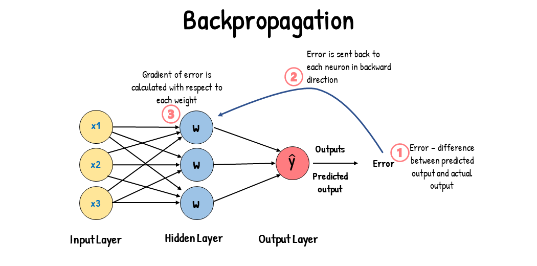
Backpropagation uses the chain rule from differential calculus to compute the gradient (or derivative) of the loss function with respect to the weights in a neural network. This gradient is then used in the gradient descent algorithm to update the weights and minimize the loss function.
Gradient descent is an optimization algorithm that uses the gradient (or derivative) of the loss function to decide in which direction to adjust the weights in order to minimize the loss. The gradient points in the direction of steepest ascent, so by moving in the opposite direction (i.e., the direction of steepest descent), the algorithm iteratively finds the minimum of the function.
## The Simple Idea Behind The Magic
At the core of many advanced technologies are simple algorithms working with lots of data. It's like teaching someone to play a song on the piano. The more they practice (data), and the more they adjust based on feedback (simple learning rules), the better they get.
### Big Data: The Fuel for Learning
Data is like the raw material for machine learning.
- **Learning from Examples**: The more data you feed into a model, the better it can learn patterns and make accurate predictions.
- **Capturing Nuances**: Large datasets help models understand subtle differences that small datasets might miss.
Imagine trying to recognize different dog breeds. If you've only seen a few pictures, you might confuse a Labrador with a Golden Retriever. But if you've seen thousands of images, you'll start to notice the unique features of each breed.
### Backpropagation and Gradient Descent: The Learning Process
These might sound technical, but they're simpler than you think.
#### Backpropagation: Learning from Mistakes
Backpropagation is how a model learns from errors.
- **Making a Guess**: The model makes a prediction based on current data.
- **Checking Accuracy**: It compares its prediction to the actual result to see how far off it was.
- **Adjusting**: It then goes back and tweaks its internal settings to improve next time.
It's like practicing basketball shots. After each shot, you see if you made it or missed. If you missed, you adjust your technique for the next shot.
#### Gradient Descent: Finding the Best Path
Gradient descent helps the model figure out the best way to adjust its settings to reduce errors.
- **Calculating Direction**: It figures out which way to change the settings to improve accuracy.
- **Taking Steps**: It makes small adjustments in that direction.
Think of it as walking downhill to reach the lowest point in a valley. Even if it's foggy and you can't see far, you can feel the slope under your feet and keep moving downward.
## The Gradient
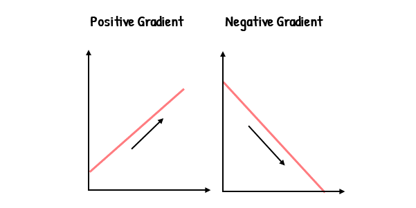
Gradient descent employs backpropagation to ascertain the direction of navigation. In particular, it utilizes the gradients computed via backpropagation. These gradients are instrumental in deciding the path to follow to locate the minimum point. Essentially, we are seeking the negative gradient. This is due to the fact that a negative gradient signifies a diminishing slope. A diminishing slope implies that moving downward will guide us to the minimum point.
## The Code: Seeing It in Action
To make this concept more concrete, let's look at a simple Python script that demonstrates how large amounts of data and simple algorithms can achieve impressive results. We'll use **PyTorch Lightning**, a user-friendly library that simplifies the training process.
### What We'll Do
We'll create a simple neural network to classify points inside or outside a circle.
- **Generate Data**: Create thousands of random points labeled based on whether they fall inside a circle.
- **Build a Model**: Use a basic neural network with one hidden layer.
- **Train the Model**: Apply backpropagation and gradient descent to teach the model.
- **Visualize the Results**: See how well the model learned by plotting the decision boundary.
### The Script Breakdown
Here's the code:
```python
# demo.py
import numpy as np
import matplotlib.pyplot as plt
from sklearn.model_selection import train_test_split
import torch
from torch.utils.data import DataLoader, TensorDataset
import pytorch_lightning as pl
from torch import nn
def generate_data(num_samples):
"""
Generate synthetic 2D data points and label them based on whether
they are inside a circle centered at (0, 0) with radius 0.5.
"""
X = np.random.uniform(-1, 1, (num_samples, 2))
Y = np.zeros((num_samples, 1), dtype=np.float32)
for i in range(num_samples):
x, y = X[i]
if x**2 + y**2 <= 0.5**2:
Y[i] = 1.0 # Inside the circle
else:
Y[i] = 0.0 # Outside the circle
return X.astype(np.float32), Y
class CircleClassifier(pl.LightningModule):
def __init__(self):
super().__init__()
self.model = nn.Sequential(
nn.Linear(2, 8),
nn.ReLU(),
nn.Linear(8, 1),
nn.Sigmoid()
)
self.loss_fn = nn.BCELoss()
def forward(self, x):
return self.model(x).squeeze()
def training_step(self, batch, batch_idx):
x, y = batch
preds = self(x)
loss = self.loss_fn(preds, y.squeeze())
self.log('train_loss', loss)
return loss
def validation_step(self, batch, batch_idx):
x, y = batch
preds = self(x)
loss = self.loss_fn(preds, y.squeeze())
acc = ((preds > 0.5) == y.squeeze()).float().mean()
self.log('val_loss', loss)
self.log('val_acc', acc, prog_bar=True)
return loss
def configure_optimizers(self):
optimizer = torch.optim.SGD(self.parameters(), lr=0.1)
return optimizer
def main():
# Step 1: Generate Data
num_samples = 5000
X, Y = generate_data(num_samples)
X_train, X_test, Y_train, Y_test = train_test_split(
X, Y, test_size=0.2, random_state=42
)
# Create DataLoaders
train_dataset = TensorDataset(torch.from_numpy(X_train), torch.from_numpy(Y_train))
test_dataset = TensorDataset(torch.from_numpy(X_test), torch.from_numpy(Y_test))
train_loader = DataLoader(train_dataset, batch_size=32)
val_loader = DataLoader(test_dataset, batch_size=32)
# Step 2: Initialize Model
model = CircleClassifier()
# Step 3: Train the Model
trainer = pl.Trainer(max_epochs=50)
trainer.fit(model, train_loader, val_loader)
# Step 4: Evaluate the Model
trainer.validate(model, val_loader)
# Step 5: Visualize the Decision Boundary
xx, yy = np.mgrid[-1:1:0.01, -1:1:0.01]
grid = np.c_[xx.ravel(), yy.ravel()]
grid_tensor = torch.from_numpy(grid.astype(np.float32))
with torch.no_grad():
probs = model(grid_tensor).reshape(xx.shape)
probs = probs.numpy()
plt.figure(figsize=(8, 6))
contour = plt.contourf(xx, yy, probs, levels=[0, 0.5, 1], cmap="RdBu", alpha=0.6)
plt.colorbar(contour)
plt.scatter(X_train[:, 0], X_train[:, 1], c=Y_train[:, 0], cmap="RdBu", edgecolors='k', alpha=0.5)
plt.title('Decision Boundary and Training Data')
plt.xlabel('X1')
plt.ylabel('X2')
plt.show()
if __name__ == '__main__':
main()
```
Let's break it down.
#### Generating Data
We create `num_samples` random points within the square from -1 to 1 on both axes.
```python
def generate_data(num_samples):
X = np.random.uniform(-1, 1, (num_samples, 2)) # Random points
Y = np.zeros((num_samples, 1), dtype=np.float32) # Labels
for i in range(num_samples):
x, y = X[i]
if x**2 + y**2 <= 0.5**2:
Y[i] = 1.0 # Inside the circle of radius 0.5
return X.astype(np.float32), Y
```
- **Purpose**: We're simulating a simple classification problem where the model needs to learn to distinguish points inside a circle from those outside.
- **Why It Matters**: This provides a visual and intuitive way to see how the model learns.
#### Building the Model with PyTorch Lightning
We define a simple neural network using PyTorch Lightning.
```python
class CircleClassifier(pl.LightningModule):
def __init__(self):
super().__init__()
self.model = nn.Sequential(
nn.Linear(2, 8), # Input layer to hidden layer
nn.ReLU(), # Activation function
nn.Linear(8, 1), # Hidden layer to output layer
nn.Sigmoid() # Output activation to get probabilities
)
self.loss_fn = nn.BCELoss() # Binary Cross Entropy Loss
def forward(self, x):
return self.model(x).squeeze()
```
- **Layers**:
- **Input Layer**: Takes two inputs (x and y coordinates).
- **Hidden Layer**: 8 neurons with ReLU activation function.
- **Output Layer**: 1 neuron with sigmoid activation to output a probability between 0 and 1.
- **Loss Function**: Binary Cross Entropy Loss measures the difference between predicted and actual labels.
- **Why Simple**: This network is straightforward, showing that even basic models can learn complex patterns with enough data.
#### Training and Validation Steps
We define how the model should train and validate.
```python
def training_step(self, batch, batch_idx):
x, y = batch
preds = self(x)
loss = self.loss_fn(preds, y.squeeze())
self.log('train_loss', loss)
return loss
def validation_step(self, batch, batch_idx):
x, y = batch
preds = self(x)
loss = self.loss_fn(preds, y.squeeze())
acc = ((preds > 0.5) == y.squeeze()).float().mean()
self.log('val_loss', loss)
self.log('val_acc', acc, prog_bar=True)
return loss
```
- **Training Step**:
- **Calculates Predictions**: Uses the model to predict outputs.
- **Computes Loss**: Measures how far off the predictions are.
- **Logs Loss**: Keeps track of the loss for monitoring.
- **Validation Step**:
- **Same as Training Step**, but also calculates accuracy to see how well the model is performing.
#### Optimizer Configuration
We specify the optimizer for gradient descent.
```python
def configure_optimizers(self):
optimizer = torch.optim.SGD(self.parameters(), lr=0.1)
return optimizer
```
- **Optimizer**: Stochastic Gradient Descent (SGD) adjusts the model parameters to minimize the loss.
- **Learning Rate**: Set to 0.1, which determines the size of each adjustment step.
#### Training the Model
We set up the training process.
```python
def main():
# Generate Data
num_samples = 5000
X, Y = generate_data(num_samples)
X_train, X_test, Y_train, Y_test = train_test_split(X, Y, test_size=0.2, random_state=42)
# Create DataLoaders
train_dataset = TensorDataset(torch.from_numpy(X_train), torch.from_numpy(Y_train))
test_dataset = TensorDataset(torch.from_numpy(X_test), torch.from_numpy(Y_test))
train_loader = DataLoader(train_dataset, batch_size=32)
val_loader = DataLoader(test_dataset, batch_size=32)
# Initialize Model
model = CircleClassifier()
# Train the Model
trainer = pl.Trainer(max_epochs=50)
trainer.fit(model, train_loader, val_loader)
```
- **DataLoaders**: Handle batching of data for training.
- **Trainer**: Manages the training loop, applying backpropagation and gradient descent under the hood.
- **Epochs**: The number of times the model will go through the entire training dataset.
#### Evaluating and Visualizing
We check the model's performance and visualize the results.
```python
# Evaluate the Model
trainer.validate(model, val_loader)
# Visualize Decision Boundary
xx, yy = np.mgrid[-1:1:0.01, -1:1:0.01]
grid = np.c_[xx.ravel(), yy.ravel()]
grid_tensor = torch.from_numpy(grid.astype(np.float32))
with torch.no_grad():
probs = model(grid_tensor).reshape(xx.shape)
probs = probs.numpy()
plt.figure(figsize=(8, 6))
contour = plt.contourf(xx, yy, probs, levels=[0, 0.5, 1], cmap="RdBu", alpha=0.6)
plt.colorbar(contour)
plt.scatter(X_train[:, 0], X_train[:, 1], c=Y_train[:, 0], cmap="RdBu", edgecolors='k', alpha=0.5)
plt.title('Decision Boundary and Training Data')
plt.xlabel('X1')
plt.ylabel('X2')
plt.show()
```
- **Validation**: Checks model performance on unseen data.
- **Decision Boundary**: Visualizes how the model separates the space into areas predicted as inside or outside the circle.
- **Data Points**: Plots the training data to see how well the model's predictions align.
---
# Appendix
## Understanding Differential Calculus
Differential calculus, a subfield of calculus, focuses on describing change. It involves the concept of a derivative, which can be interpreted as the rate of change of a function at a point. In other words, it measures how a function changes as its input changes. This concept is fundamental to understanding how things change over time and is at the heart of many scientific and mathematical disciplines.
## The Impact of Differential Calculus
Differential calculus has had a profound impact on our understanding of the world and the development of modern technology. It is fundamental to physics, engineering, computer science, economics, statistics, and many other fields.
In physics, for example, differential calculus is used to describe the motion of objects, the behavior of electric and magnetic fields, the propagation of light, and much more. It allows us to predict how physical systems will evolve over time based on their current state.
## Newton, Einstein, and the Evolution of Physics
Sir Isaac Newton, one of the inventors of calculus, used it to formulate his laws of motion and universal gravitation, laying the groundwork for classical physics. Newton's laws describe the motion of objects in our everyday world with great accuracy. His work was a monumental leap in human understanding, and Albert Einstein once said of Newton's contributions, "perhaps the greatest advance in thought that a single individual was ever privileged to make."
However, at the turn of the 20th century, Albert Einstein showed that Newton's laws break down when dealing with very high speeds or very strong gravitational fields. Einstein's theory of relativity, which describes the behavior of objects at high speeds and the nature of gravity, required a more advanced form of calculus known as tensor calculus.
### FULL CODE
```python
# demo.py
import numpy as np
import matplotlib.pyplot as plt
from sklearn.model_selection import train_test_split
import torch
from torch.utils.data import DataLoader, TensorDataset
import pytorch_lightning as pl
from torch import nn
def generate_data(num_samples):
"""
Generate synthetic 2D data points and label them based on whether
they are inside a circle centered at (0, 0) with radius 0.5.
"""
X = np.random.uniform(-1, 1, (num_samples, 2))
Y = np.zeros((num_samples, 1), dtype=np.float32)
for i in range(num_samples):
x, y = X[i]
if x**2 + y**2 <= 0.5**2:
Y[i] = 1.0 # Inside the circle
else:
Y[i] = 0.0 # Outside the circle
return X.astype(np.float32), Y
class CircleClassifier(pl.LightningModule):
def __init__(self):
super().__init__()
self.model = nn.Sequential(
nn.Linear(2, 8),
nn.ReLU(),
nn.Linear(8, 1),
nn.Sigmoid()
)
self.loss_fn = nn.BCELoss()
def forward(self, x):
return self.model(x).squeeze()
def training_step(self, batch, batch_idx):
x, y = batch
preds = self(x)
loss = self.loss_fn(preds, y.squeeze())
self.log('train_loss', loss)
return loss
def validation_step(self, batch, batch_idx):
x, y = batch
preds = self(x)
loss = self.loss_fn(preds, y.squeeze())
acc = ((preds > 0.5) == y.squeeze()).float().mean()
self.log('val_loss', loss)
self.log('val_acc', acc, prog_bar=True)
return loss
def configure_optimizers(self):
optimizer = torch.optim.SGD(self.parameters(), lr=0.1)
return optimizer
def main():
# Step 1: Generate Data
num_samples = 5000
X, Y = generate_data(num_samples)
X_train, X_test, Y_train, Y_test = train_test_split(
X, Y, test_size=0.2, random_state=42
)
# Create DataLoaders
train_dataset = TensorDataset(torch.from_numpy(X_train), torch.from_numpy(Y_train))
test_dataset = TensorDataset(torch.from_numpy(X_test), torch.from_numpy(Y_test))
train_loader = DataLoader(train_dataset, batch_size=32)
val_loader = DataLoader(test_dataset, batch_size=32)
# Step 2: Initialize Model
model = CircleClassifier()
# Step 3: Train the Model
trainer = pl.Trainer(max_epochs=50)
trainer.fit(model, train_loader, val_loader)
# Step 4: Evaluate the Model
trainer.validate(model, val_loader)
# Step 5: Visualize the Decision Boundary
xx, yy = np.mgrid[-1:1:0.01, -1:1:0.01]
grid = np.c_[xx.ravel(), yy.ravel()]
grid_tensor = torch.from_numpy(grid.astype(np.float32))
with torch.no_grad():
probs = model(grid_tensor).reshape(xx.shape)
probs = probs.numpy()
plt.figure(figsize=(8, 6))
contour = plt.contourf(xx, yy, probs, levels=[0, 0.5, 1], cmap="RdBu", alpha=0.6)
plt.colorbar(contour)
plt.scatter(X_train[:, 0], X_train[:, 1], c=Y_train[:, 0], cmap="RdBu", edgecolors='k', alpha=0.5)
plt.title('Decision Boundary and Training Data')
plt.xlabel('X1')
plt.ylabel('X2')
plt.show()
if __name__ == '__main__':
main()
"""
┏━━━━━━━━━━━━━━━━━━━━━━━━━━━┳━━━━━━━━━━━━━━━━━━━━━━━━━━━┓
┃ Validate metric ┃ DataLoader 0 ┃
┡━━━━━━━━━━━━━━━━━━━━━━━━━━━╇━━━━━━━━━━━━━━━━━━━━━━━━━━━┩
│ val_acc │ 0.9890000224113464 │
│ val_loss │ 0.056591153144836426 │
└───────────────────────────┴───────────────────────────┘
"""
```