https://github.com/ranfysvalle02/rl-basics
Teaching an agent to navigate a maze using Q-learning.
https://github.com/ranfysvalle02/rl-basics
Last synced: 7 months ago
JSON representation
Teaching an agent to navigate a maze using Q-learning.
- Host: GitHub
- URL: https://github.com/ranfysvalle02/rl-basics
- Owner: ranfysvalle02
- Created: 2025-01-12T23:07:45.000Z (9 months ago)
- Default Branch: main
- Last Pushed: 2025-01-13T20:44:14.000Z (9 months ago)
- Last Synced: 2025-01-22T21:19:03.799Z (9 months ago)
- Language: Python
- Homepage:
- Size: 1.22 MB
- Stars: 0
- Watchers: 1
- Forks: 0
- Open Issues: 0
-
Metadata Files:
- Readme: README.md
Awesome Lists containing this project
README
# reinforcement-learning-basics

---
# **Maze Mastery with Q-Learning**
*Have you ever been lost in a maze and wished for a strategy to find your way out? What if a computer could learn to solve the maze by itself? Let's dive into the exciting world of reinforcement learning and see how we can teach a computer to navigate a maze using Q-learning!*
---
## Introduction
Imagine a tiny robot placed at the entrance of a maze. It doesn't know where to go at first, but with experience, it learns the best path to the exit. This learning process is similar to how we learn—by trying different things, making mistakes, and figuring out what works best.
In this guide, we'll explore how reinforcement learning helps a computer (our robot agent) learn to solve a maze. We'll explain the concepts in a fun and simple way, perfect for anyone curious about artificial intelligence!
---
## What is Reinforcement Learning?
Reinforcement learning is like training a pet through rewards and penalties. Suppose you're teaching a dog to sit:
- **Reward**: When the dog sits on command, you give it a treat.
- **No Reward/Penalty**: If the dog doesn't sit, you don't give it a treat or say "no."
Over time, the dog learns that sitting when told leads to a tasty treat!
Similarly, in reinforcement learning, we have:
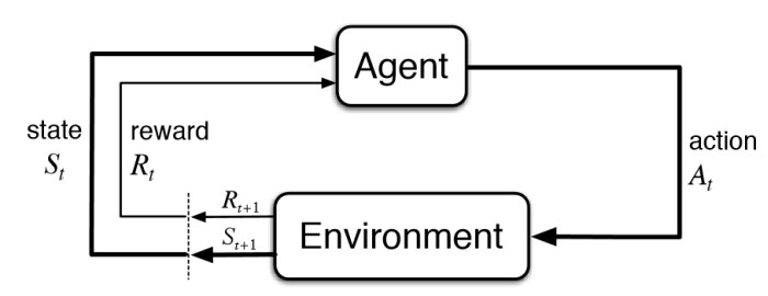
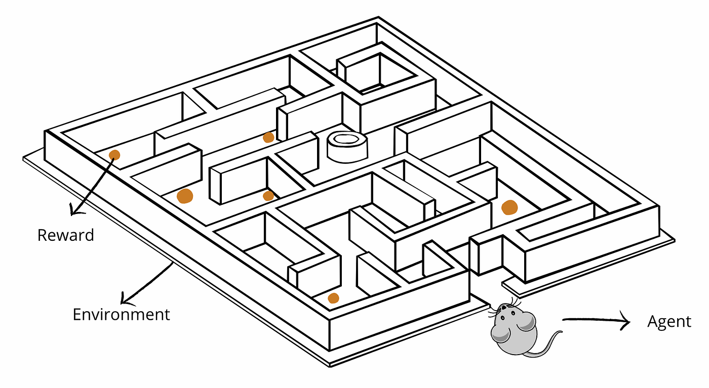
- **Agent**: The learner or decision-maker (our computer program).
- **Environment**: The world the agent interacts with (the maze).
- **Actions**: What the agent can do (move up, down, left, right).
- **Rewards**: Feedback from the environment (positive for good actions, negative for bad ones).
The agent learns by taking actions, receiving rewards or penalties, and updating its behavior to maximize the total reward.
### **Core Concepts in Reinforcement Learning**
#### **1. Policy**
- **Definition:** A policy is the agent's strategy or rulebook for choosing actions in each state. It's what guides the agent's behavior.
- **Goal:** The objective in reinforcement learning is to find the optimal policy that maximizes the agent's total reward over time.
#### **2. Value Functions**
Value functions estimate how good it is for the agent to be in a certain state, considering future rewards. They help the agent evaluate the potential long-term benefit of states and actions.
- **State-Value Function:** Estimates the expected total reward starting from a state and following a particular policy.
- **Action-Value Function (Q-Value):** Estimates the expected total reward starting from a state, taking a specific action, and then following a policy.
#### **3. The Balance Between Exploration and Exploitation**
One of the central challenges in reinforcement learning is deciding between:
- **Exploration:** Trying new actions to discover their effects, which might lead to higher rewards in the future.
- **Exploitation:** Using known actions that have provided high rewards in the past to maximize immediate reward.
**Balancing Both:**
- **Epsilon-Greedy Strategy:** A common approach where the agent mostly chooses the best-known action (exploitation) but occasionally tries a random action (exploration). This helps the agent continue learning about the environment and avoid missing out on potentially better actions.
#### **4. Rewards and Their Role**
- **Positive Rewards:** Encourage the agent to repeat actions that lead to good outcomes.
- **Negative Rewards (Penalties):** Discourage the agent from taking actions that lead to bad outcomes.
**Designing Rewards:**
- The reward system must be carefully designed to align with the desired goals. In our maze example, reaching the goal gives a high positive reward, while hitting a wall incurs a penalty.
#### **5. Learning from Experience**
- **Trial and Error:** The agent learns by trying actions and seeing the results, much like how humans learn.
- **Updating Knowledge:** After each action, the agent updates its understanding of the environment, which improves its future decisions.
---
### **Why These Concepts Matter**
Understanding these fundamentals helps us grasp how reinforcement learning agents operate:
- **MDPs Provide Structure:** They define the environment and rules within which the agent learns.
- **Policies Guide Actions:** They determine how the agent behaves in each state.
- **Value Functions and Q-Learning Drive Learning:** They enable the agent to evaluate actions and learn optimal behavior through experience.
- **Exploration Is Key for Learning:** Trying new actions helps the agent discover better strategies.
- **Rewards Shape Behavior:** They motivate the agent to achieve the desired outcomes.
---
## Understanding Q-Learning Fundamentals
### What is Q-Learning?
Q-learning is a type of reinforcement learning algorithm. It helps the agent learn the value of taking a certain action in a particular state (position in the maze).
- **Q-Value (Quality Value)**: A number that represents the expected future rewards for taking an action from a specific state.
- **Q-Table**: A table where the agent stores Q-values for every possible state-action pair.
Think of the Q-table as a big map or memory that tells the agent the best action to take from any position in the maze based on past experiences.
### How Does Q-Learning Work?
1. **Initialize the Q-Table**: Fill it with zeros. The agent knows nothing at the start.
2. **Observe the Current State**: The agent looks at where it is in the maze.
3. **Choose an Action**: Decide whether to explore new actions or exploit known ones.
4. **Perform the Action**: Move in the chosen direction.
5. **Receive a Reward**: Get feedback (positive or negative) based on the action.
6. **Update the Q-Table**: Adjust the Q-value for the state-action pair using the Q-learning formula.
7. **Repeat**: Continue the process until the goal is reached or a maximum number of steps is taken.
---
## Our Maze Adventure
Let's set up our maze and teach the agent to navigate it!
### The Maze Layout
We'll define a simple maze using a grid:
```python
maze = [
[0, 0, 0, 0, 0], # 0 represents a wall
[0, 1, 1, 1, 0], # 1 represents a path
[0, 1, 9, 1, 0], # 9 represents the goal
[0, 1, 1, 1, 0],
[0, 0, 0, 0, 0]
]
```
- **Walls (0)**: Places the agent cannot move into.
- **Paths (1)**: Open spaces where the agent can move.
- **Goal (9)**: The target position the agent aims to reach.
**Visual Representation:**
```
█ █ █ █ █
█ . . . █
█ . G . █
█ . . . █
█ █ █ █ █
```
- `█`: Wall
- `. `: Path
- `G`: Goal
### Getting Ready to Learn
We set up the maze dimensions and possible actions:
```python
maze_height = len(maze)
maze_width = len(maze[0])
actions = ['up', 'down', 'left', 'right']
```
Create the Q-table (the agent's memory):
```python
q_table = np.zeros((maze_height, maze_width, len(actions)))
```
Set the learning parameters (hyperparameters):
- **Alpha (Learning Rate)**: How much new information overrides old information (set to 0.1).
- **Gamma (Discount Factor)**: Importance of future rewards (set to 0.9).
- **Epsilon (Exploration Rate)**: How often to explore versus exploit (set to 0.1).
- **Episodes**: Number of training cycles (set to 1000).
---
## Training the Agent
### The Code: Setting Up
Here's the full code that we'll walk through:
```python
import numpy as np
import random
# Define the maze
maze = [
[0, 0, 0, 0, 0], # 0 represents a wall
[0, 1, 1, 1, 0], # 1 represents a path
[0, 1, 9, 1, 0], # 9 represents the goal
[0, 1, 1, 1, 0],
[0, 0, 0, 0, 0]
]
# Maze dimensions
maze_height = len(maze)
maze_width = len(maze[0])
# Actions the agent can take
actions = ['up', 'down', 'left', 'right']
# Create a Q-table initialized to zeros
q_table = np.zeros((maze_height, maze_width, len(actions)))
# Hyperparameters
alpha = 0.1 # Learning rate
gamma = 0.9 # Discount factor
epsilon = 0.1 # Exploration rate
episodes = 1000 # Number of times the agent tries to learn
# Starting position
start_position = (1, 1)
# Function to get the next position based on the action
def get_next_position(position, action):
x, y = position
if action == 'up':
x -= 1
elif action == 'down':
x += 1
elif action == 'left':
y -= 1
elif action == 'right':
y += 1
return (x, y)
```
### Exploration vs. Exploitation: The Balancing Act
One of the key challenges in reinforcement learning is deciding between:
- **Exploration**: Trying new actions to discover their effects.
- **Exploitation**: Using known actions that give the highest rewards.
#### A Detailed Example
Imagine you're at an ice cream shop with many flavors:
- **Exploration**: You try a new flavor you've never had before. It might become your new favorite or you might not like it at all.
- **Exploitation**: You order your usual favorite flavor. You know you'll enjoy it, but you won't discover anything new.
In our maze, the agent faces a similar choice at each step:
- **Should it try a new direction (exploration), possibly finding a better path or hitting a wall?**
- **Or should it go the way it knows leads to good rewards (exploitation)?**
We use the **epsilon-greedy strategy** to balance exploration and exploitation:
```python
# Decide whether to explore or exploit
if random.uniform(0, 1) < epsilon:
# Explore: choose a random action
action = random.choice(actions)
print(f"Episode {episode}: Exploring action '{action}' at position {position}.")
else:
# Exploit: choose the best action from Q-table
action_index = np.argmax(q_table[x, y])
action = actions[action_index]
print(f"Episode {episode}: Exploiting action '{action}' at position {position}.")
```
- **Epsilon (ε)**: A small number (e.g., 0.1) representing the chance to explore.
- **If a random number between 0 and 1 is less than ε**, the agent explores.
- **Otherwise**, it exploits what it has learned.
#### Why Balance Both?
- **Exploration** is crucial in the beginning so the agent can learn about the environment.
- **Exploitation** uses the knowledge gained to make the best decisions.
### Moving Through the Maze
The agent moves based on the chosen action:
```python
def get_next_position(position, action):
x, y = position
if action == 'up':
x -= 1
elif action == 'down':
x += 1
elif action == 'left':
y -= 1
elif action == 'right':
y += 1
return (x, y)
```
We then check what happens after the move:
- **Hit a Wall or Boundary**:
- The agent receives a negative reward (-1).
- It stays in the same place because it can't move into a wall.
- **Reached the Goal**:
- The agent receives a positive reward (10).
- The episode ends since the goal is reached.
- **Moved to an Open Path**:
- The agent receives a small negative reward (-0.1).
- This encourages the agent to find the shortest path (so it doesn't wander aimlessly).
### Updating the Q-Table
After receiving the reward, the agent updates its Q-table:
```python
# Update Q-table
action_index = actions.index(action)
old_value = q_table[x, y, action_index]
next_max = np.max(q_table[x_next, y_next])
# Q-learning formula
new_value = (1 - alpha) * old_value + alpha * (reward + gamma * next_max)
q_table[x, y, action_index] = new_value
```
**Let's Break Down the Q-learning Formula:**
- **Old Value**: The existing Q-value for the current state and action.
- **Reward**: The immediate reward received after taking the action.
- **Next Max**: The maximum Q-value for the next state (the best future reward).
- **Alpha (α)**: Learning rate determining how much new information overrides old information.
- **Gamma (γ)**: Discount factor determining the importance of future rewards (closer to 1 means future rewards are highly valued).
The formula updates the Q-value to be a combination of:
- What the agent already knew (**old_value**).
- What it just learned (**reward + gamma * next_max**).
This way, the agent learns the expected utility of taking an action from a state, considering both immediate and future rewards.
### The Training Loop
Putting it all together, here's how we train the agent over multiple episodes:
```python
print("Starting Q-learning training...")
# Training the agent
for episode in range(episodes):
position = start_position
done = False
while not done:
x, y = position
# Exploration vs. Exploitation (as discussed earlier)
# Get the next position based on the action
next_position = get_next_position(position, action)
x_next, y_next = next_position
# Check the result of the action (as discussed earlier)
# Update Q-table (as discussed earlier)
# Move to the next position
position = next_position
print("\nTraining completed.")
```
---
## Finding the Best Path
After training, the agent uses the learned Q-table to find the optimal path to the goal without exploring (epsilon is effectively 0).
### The Code: Navigating the Maze
```python
# After training, find the best path
position = start_position
done = False
path = [position]
print("\nFinding the best path based on the learned Q-table...")
while not done:
x, y = position
# Choose the best action based on the learned Q-table
action_index = np.argmax(q_table[x, y])
action = actions[action_index]
next_position = get_next_position(position, action)
x_next, y_next = next_position
# Check if the next move leads to the goal
if maze[x_next][y_next] == 9:
path.append(next_position)
print(f"Moved '{action}' to {next_position}. Goal reached!")
done = True
elif maze[x_next][y_next] == 0 or x_next < 0 or x_next >= maze_height or y_next < 0 or y_next >= maze_width:
print(f"Encountered a wall or boundary when moving '{action}'. Cannot proceed further.")
done = True
else:
position = next_position
path.append(position)
print(f"Moved '{action}' to {position}.")
# Print the path taken
print("\nPath to the goal:")
for step in path:
print(step)
```
### How the Agent Finds the Best Path
- **Selects the Best Action**: At each position, the agent picks the action with the highest Q-value.
- **Avoids Exploration**: Since it's using the learned Q-table, it no longer explores randomly.
- **Efficient Navigation**: It moves directly towards the goal based on what it has learned.
---
## Why This Works
### Learning from Experience
The agent improves over time by:
- **Receiving Rewards**:
- Positive rewards for actions that lead towards the goal.
- Negative rewards for hitting walls or boundaries.
- **Updating the Q-Table**:
- Adjusting its understanding of which actions are good or bad in each state.
### Mimicking Human Learning
Just like how we learn from our experiences:
- **Trial and Error**: Trying different paths and learning from mistakes.
- **Remembering**: Keeping track of what works and what doesn't.
- **Optimizing Behavior**: Choosing actions that lead to better outcomes based on past experiences.
---
## Key Takeaways
- **Reinforcement Learning**: A way for agents to learn by interacting with an environment and receiving feedback.
- **Q-Learning**: An algorithm that helps agents learn the value of actions in specific states to maximize rewards.
- **Exploration vs. Exploitation**: Balancing the need to try new things and using known information to make the best decisions.
- **Agent's Goal**: To maximize total rewards by choosing the best actions, ultimately learning the optimal path to the goal.
---
## Try It Yourself!
You can run the provided Python code and watch the agent learn to solve the maze!
Here are some fun experiments:
- **Change the Maze Layout**:
- Add more walls or paths to make the maze more challenging.
- Move the goal to a different position.
- **Adjust Learning Parameters**:
- Change **alpha**, **gamma**, or **epsilon** to see how it affects learning.
- For example, increase **epsilon** to see more exploration.
- **Increase Episodes**:
- Train the agent for more episodes to see if it improves performance.
- Observe how learning stabilizes over time.
---
## Appendix: Diving Deeper into Q-Learning
### Hyperparameters and Their Roles
- **Alpha (Learning Rate)**:
- Controls how much newly acquired information overrides old information.
- **High Alpha**: Fast learning but can overshoot optimal values.
- **Low Alpha**: Slow learning but more stable.
- **Gamma (Discount Factor)**:
- Determines the importance of future rewards.
- **Gamma close to 1**: Future rewards are emphasized.
- **Gamma close to 0**: Immediate rewards are prioritized.
- **Epsilon (Exploration Rate)**:
- Controls the likelihood of exploring new actions.
- **High Epsilon**: More exploration.
- **Low Epsilon**: More exploitation.
### Balancing Exploration and Exploitation
To optimize learning:
- **Start with High Exploration**:
- Set a higher epsilon value initially to allow the agent to learn about the environment.
- **Reduce Epsilon Over Time**:
- Gradually decrease epsilon to shift from exploration to exploitation.
- **Example**:
```python
epsilon = max(min_epsilon, epsilon * decay_rate)
```
- **min_epsilon**: The minimum exploration rate.
- **decay_rate**: How quickly exploration decreases.
### Challenges and Considerations
- **State Space Size**:
- Complex environments have a larger number of states, making the Q-table large.
- **Learning Rate Tuning**:
- Finding the right values for alpha, gamma, and epsilon is crucial for efficient learning.
- **Changing Environments**:
- If the maze changes, the agent may need to relearn the optimal path.
### Real-World Applications
Reinforcement learning has a wide range of applications across various domains:
* **Robotics:**
* **Autonomous Vehicles:** Navigating traffic, changing lanes, avoiding obstacles.
* **Industrial Robotics:** Optimizing assembly lines, improving material handling, enhancing robot dexterity.
* **Game Playing:**
* **Video Games:** Achieving superhuman performance in complex games like Go and StarCraft II.
* **Game AI:** Creating more challenging and engaging AI opponents.
* **Finance:**
* **Algorithmic Trading:** Analyzing market data, identifying trading opportunities, and executing trades automatically.
* **Portfolio Management:** Optimizing investment portfolios by balancing risk and reward.
* **Healthcare:**
* **Drug Discovery:** Accelerating the drug discovery process by optimizing the design of new molecules.
* **Personalized Medicine:** Developing personalized treatment plans for patients.
* **Recommendation Systems:**
* **Product Recommendations:** Personalizing recommendations for users on platforms like Netflix and Amazon.
* **Content Recommendations:** Tailoring content recommendations to individual user preferences on social media and news platforms.
---
### **Markov Decision Process (MDP)**
A **Markov Decision Process (MDP)** is a mathematical framework used to describe the environment in reinforcement learning. It provides a way to model decision-making where outcomes are partly random and partly under the control of the decision-maker (the agent).
**Key Components of an MDP:**
1. **States (S):** All the possible situations the agent can be in. In our maze example, each position in the maze grid represents a state.
2. **Actions (A):** All the possible moves the agent can make from each state. In the maze, these are moving up, down, left, or right.
3. **Transitions:** The rules that describe what happens when the agent takes an action in a state. It defines the next state the agent will end up in after taking an action.
4. **Rewards (R):** Feedback the agent receives after transitioning to a new state because of an action. Rewards guide the agent toward good behavior by assigning positive values for desirable outcomes and negative values for undesirable ones.
5. **Policy (π):** The strategy that the agent uses to decide what action to take in each state. It's like a set of instructions or a map that tells the agent the best action to choose.
**The Markov Property:**
An important feature of MDPs is the **Markov Property**, which means that the future state depends only on the current state and the action taken, not on any past states or actions. In other words, the process doesn't have memory of past events beyond the current situation.
---
### **Understanding Q-Learning in the Context of MDPs**
**Q-Learning** is a reinforcement learning algorithm that allows an agent to learn the optimal actions to take in any state, without needing a model of the environment (meaning the agent doesn't need to know the transition rules beforehand).
**How Q-Learning Relates to MDPs:**
- **States and Actions:** Q-learning evaluates the quality (Q-value) of taking a certain action in a specific state.
- **Rewards:** The agent updates its knowledge based on the rewards received after taking actions.
- **Policy:** Over time, as the Q-values get updated, the agent develops a policy that tells it the best action to take from each state to maximize its total reward.
---
## **Conclusion**
Reinforcement learning allows computers to learn from experiences, much like humans do. By teaching an agent to navigate a maze using Q-learning, we've seen how simple concepts can lead to powerful learning.
Whether you're new to programming or just curious about how AI works, experimenting with reinforcement learning is a fun way to explore the field!
---
*Remember, learning is a journey filled with trial and error. Just like our agent, keep exploring, and you'll find your way to success!*
---
---
# **Addendum: The Role of Calculus in Advanced Q-Learning**
In our exploration of teaching an agent to navigate a maze using Q-learning, we utilized simple calculations and a straightforward Q-table. This method works wonderfully for small, discrete environments. But what happens when our agent enters a more complex world with countless possibilities? Here, we step into the realm where calculus becomes a crucial tool.
---
## **From Q-Tables to Neural Networks: Handling Complexity**
Imagine trying to teach our agent to navigate an entire city rather than a small maze. The number of possible positions and actions skyrockets, making it impractical to use a table to store every possible Q-value.
To overcome this, we use **function approximation** with tools like **neural networks**. Instead of a table, the agent now has a flexible model that can estimate Q-values for any given state.
---
## **Learning to Learn: Where Calculus Comes In**
Training a neural network involves adjusting its internal parameters (weights and biases) to make better predictions. But how does the network know which way to adjust these parameters? This is where calculus, specifically the concept of **gradients**, plays a key role.
### **Analogy: Finding the Fastest Route Downhill**
Imagine you're standing on a hill in a fog, trying to find the quickest way down:
- **Feeling the Slope**: You can't see far, but you can feel which direction slopes downward the most.
- **Taking a Step**: You take small steps in that direction.
- **Re-evaluating**: At each step, you reassess the slope and adjust your path.
Calculus helps the neural network do the same — it calculates the "slope" of the error with respect to its parameters and adjusts them to reduce this error, effectively finding the fastest route to better predictions.
---
## **Gradient Descent: The Agent's Guide**
- **Calculating the Error**: The network compares its predicted Q-values with the actual rewards.
- **Determining the Direction**: Using gradients, it figures out which way to adjust the parameters to reduce the error.
- **Updating Parameters**: It takes small steps (adjustments) in that direction.
- **Iterating**: This process repeats, gradually improving the network's predictions.
---
## **Empowering the Agent in Complex Environments**
By incorporating calculus and neural networks:
- **Generalization**: The agent can handle new, unseen states by estimating Q-values on the fly.
- **Efficiency**: It’s feasible to learn in environments where storing a Q-table is impossible.
- **Advanced Capabilities**: Enables tackling tasks like image recognition, language understanding, and complex decision-making.
---
## **Why This Matters**
Understanding the role of calculus in Q-learning allows us to:
- **Build Smarter Agents**: Capable of learning and adapting in real-time.
- **Tackle Real-World Problems**: Such as autonomous driving, robotics, and more.
- **Advance AI Research**: Pushing the boundaries of what's possible with intelligent systems.
---
## **Key Takeaways**
- **Calculus Enables Advanced Learning**: It provides the mathematical foundation for training neural networks.
- **From Discrete to Continuous**: The agent moves from simple table lookups to mastering continuous environments.
- **Equipping the Agent with Intuition**: Much like humans, the agent develops an "intuition" for navigating complex scenarios.
---
*By integrating calculus into Q-learning through neural networks, we unlock the potential for agents to learn and operate in sophisticated, dynamic environments. This synergy between simple learning rules and advanced mathematics paves the way for the exciting future of artificial intelligence.*