https://github.com/ranfysvalle02/rnn-4-stocks
A repository showcasing the application of Recurrent Neural Networks (RNNs) and Long Short-Term Memory (LSTMs) for stock price prediction.
https://github.com/ranfysvalle02/rnn-4-stocks
Last synced: 6 months ago
JSON representation
A repository showcasing the application of Recurrent Neural Networks (RNNs) and Long Short-Term Memory (LSTMs) for stock price prediction.
- Host: GitHub
- URL: https://github.com/ranfysvalle02/rnn-4-stocks
- Owner: ranfysvalle02
- Created: 2024-10-21T01:50:03.000Z (12 months ago)
- Default Branch: main
- Last Pushed: 2024-10-21T02:16:47.000Z (12 months ago)
- Last Synced: 2025-04-12T21:45:02.271Z (6 months ago)
- Language: Python
- Homepage:
- Size: 56.6 KB
- Stars: 0
- Watchers: 1
- Forks: 0
- Open Issues: 0
-
Metadata Files:
- Readme: README.md
Awesome Lists containing this project
README
# rnn-4-stocks
**Disclaimer:** The use of LSTMs or any other machine learning model for stock price prediction should be considered as a tool to assist in decision-making, not as a guaranteed predictor of future returns. Investors should conduct thorough research, consider multiple factors, and exercise caution when relying on machine learning models for investment decisions.
## What Are Recurrent Neural Networks (RNNs)?
RNNs are a class of neural networks designed to recognize patterns in sequences of data, such as time series, text, or speech. Unlike traditional feedforward neural networks, RNNs have connections that form directed cycles, allowing information to persist across steps in a sequence. This architecture enables RNNs to maintain a form of memory, making them adept at tasks where context and sequence order are crucial.
### Key Characteristics of RNNs:
- **Sequential Data Handling:** Capable of processing inputs of varying lengths.
- **Shared Weights:** The same weights are applied across different time steps, reducing the number of parameters.
- **Internal State:** Maintains a hidden state that captures information about previous inputs.
## The Challenge: Vanishing and Exploding Gradients
While RNNs are powerful, they suffer from training difficulties due to the **vanishing and exploding gradient problems**. When training RNNs using backpropagation through time, gradients can become excessively small or large, making it hard for the network to learn long-term dependencies.
## Enter LSTM: Long Short-Term Memory Networks
**LSTM** networks are a special kind of RNN architecture designed to overcome the vanishing gradient problem. Introduced by Hochreiter and Schmidhuber in 1997, LSTMs have become the de facto standard for many sequential data tasks.
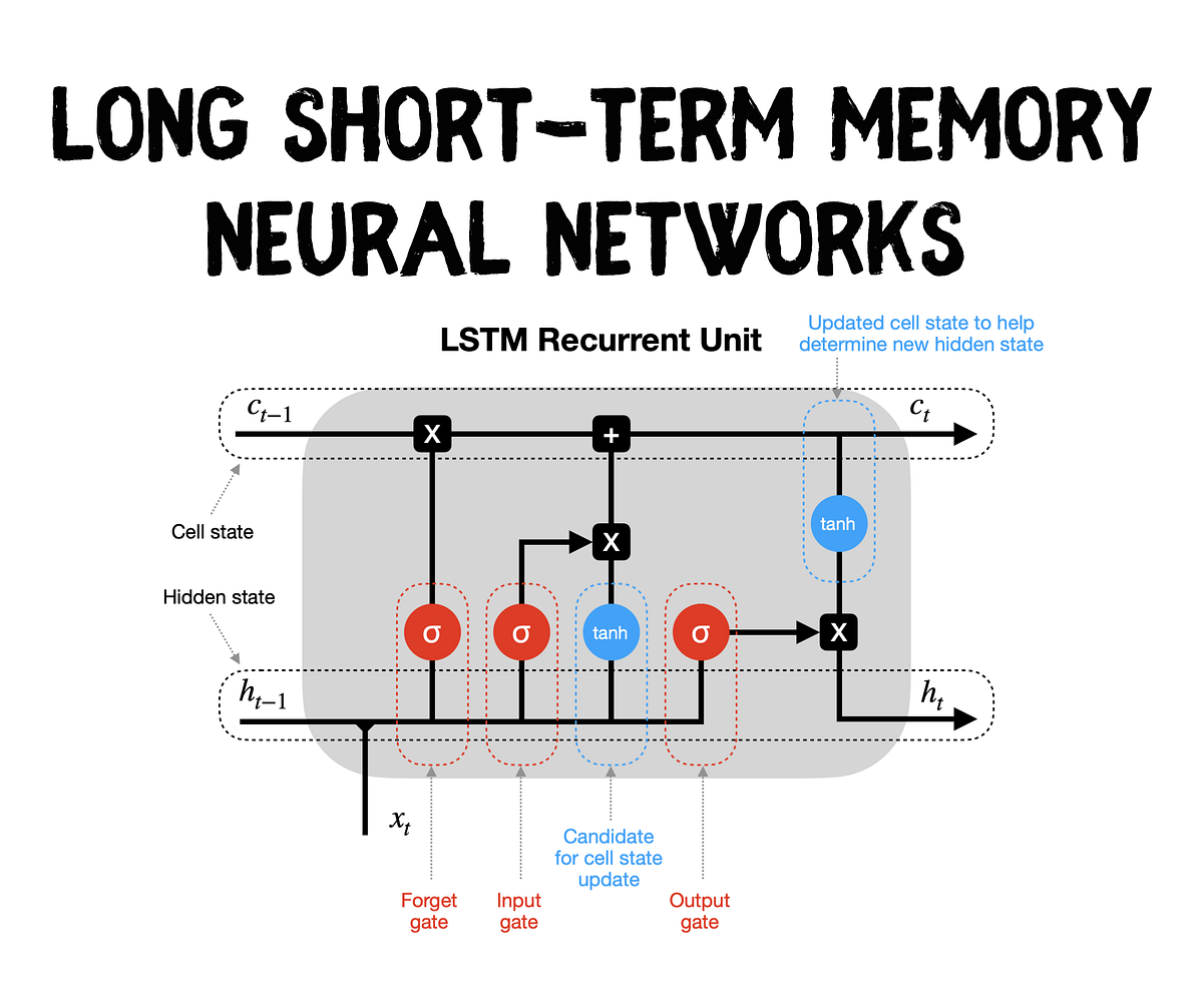
### How LSTM Works
An LSTM unit consists of several components called **gates** that regulate the flow of information:
1. **Forget Gate:** Decides what information to discard from the cell state.
2. **Input Gate:** Determines which new information to add to the cell state.
3. **Cell State:** Acts as the memory of the network, carrying relevant information across time steps.
4. **Output Gate:** Decides what part of the cell state to output.
Here's a simplified diagram of an LSTM cell:
```
Input x_t and previous hidden state h_{t-1}
|
Forget Gate
|
Input Gate --- New Candidate Values
|
Update Cell State
|
Output Gate
|
Hidden State h_t
```
By carefully managing the flow of information through these gates, LSTMs can capture long-term dependencies and retain important information over extended sequences.
### Why LSTM Matters for RNNs
LSTMs address the fundamental limitation of vanilla RNNs by maintaining a more stable gradient during training. This stability allows LSTMs to learn dependencies over longer sequences, making them suitable for complex tasks like language translation, speech recognition, and financial time series forecasting.
## Hyperparameters in RNNs and LSTMs
Choosing the right hyperparameters is crucial for the performance of RNNs and LSTMs. Here are some key hyperparameters to consider:
1. **Hidden Size:** The number of neurons in the hidden layer. A larger hidden size can capture more complex patterns but may lead to overfitting.
2. **Number of Layers:** Stacking multiple LSTM layers can help in learning hierarchical representations but increases computational complexity.
3. **Sequence Length (SEQ_LENGTH):** The length of input sequences. Longer sequences provide more context but require more memory and computational power.
4. **Learning Rate:** Controls the step size during optimization. A learning rate that's too high can cause the model to converge too quickly to a suboptimal solution, while a rate that's too low can make training painfully slow.
5. **Batch Size:** The number of samples processed before the model is updated. Larger batch sizes can stabilize training but require more memory.
6. **Dropout Rate:** Helps prevent overfitting by randomly dropping units during training.
## Training RNNs and LSTMs
Training RNNs and LSTMs involves several steps:
1. **Data Preparation:** Sequential data needs to be formatted into input-output pairs. For example, in time series forecasting, past `n` time steps are used to predict the next time step.
2. **Scaling:** Normalizing data helps in faster and more stable training.
3. **Loss Function:** Typically, Mean Squared Error (MSE) is used for regression tasks, while Cross-Entropy Loss is used for classification.
4. **Optimizer:** Algorithms like Adam or AdamW are commonly used due to their efficiency in handling sparse gradients and adaptive learning rates.
5. **Training Loop:** Involves forward pass, loss computation, backward pass, and weight updates.
Proper handling of these aspects ensures that the model learns effectively from the data.
## Practical Implementation: Stock Price Prediction with LSTM
To illustrate the concepts discussed, let's walk through a practical implementation of an LSTM model using PyTorch Lightning. This example focuses on predicting synthetic stock prices, showcasing how LSTMs can be applied to financial time series data.
### Setting Up the Environment
First, ensure you have the necessary libraries installed:
```bash
pip install numpy torch pytorch-lightning scikit-learn
```
### Generating Synthetic Stock Data
We'll start by generating synthetic stock data with reduced noise to simulate stock price movements.
```python
import numpy as np
def generate_synthetic_stock_data(seq_length, total_samples):
x = np.linspace(0, total_samples, total_samples)
stock_prices = np.sin(0.02 * x) + np.random.normal(scale=0.1, size=total_samples)
return stock_prices
TOTAL_SAMPLES = 1000
SEQ_LENGTH = 50 # Increased sequence length for more context
stock_prices = generate_synthetic_stock_data(SEQ_LENGTH, TOTAL_SAMPLES)
```
### Preparing the Dataset
Next, we'll create a custom `Dataset` class to handle our data. This includes scaling the data and generating input-output pairs.
```python
from torch.utils.data import Dataset
from sklearn.preprocessing import StandardScaler
import torch
class StockPriceDataset(Dataset):
def __init__(self, data, seq_length):
self.data = data
self.seq_length = seq_length
# Scale the data
self.scaler = StandardScaler()
self.scaled_data = self.scaler.fit_transform(self.data.reshape(-1, 1)).flatten()
def __len__(self):
return len(self.scaled_data) - self.seq_length
def __getitem__(self, idx):
seq = self.scaled_data[idx:idx + self.seq_length]
target = self.scaled_data[idx + self.seq_length]
seq = torch.tensor(seq, dtype=torch.float32).unsqueeze(1) # Shape: (seq_length, 1)
target = torch.tensor(target, dtype=torch.float32)
return seq, target
def inverse_transform(self, data):
return self.scaler.inverse_transform(data.reshape(-1, 1)).flatten()
```
### Splitting the Dataset
We'll split the dataset into training and testing sets.
```python
from torch.utils.data import random_split, DataLoader
TEST_SIZE = 100 # Size of the test set
dataset = StockPriceDataset(stock_prices, SEQ_LENGTH)
train_size = len(dataset) - TEST_SIZE
train_dataset, test_dataset = random_split(dataset, [train_size, TEST_SIZE])
train_loader = DataLoader(train_dataset, batch_size=64, shuffle=True)
val_loader = DataLoader(test_dataset, batch_size=64)
```
### Defining the LSTM Model
Using PyTorch Lightning, we'll define an LSTM model with increased complexity to better capture the underlying patterns in the data.
```python
import pytorch_lightning as pl
from torch import nn
class StockPriceLSTM(pl.LightningModule):
def __init__(self, input_size=1, hidden_size=128, num_layers=3, output_size=1, learning_rate=0.001):
super(StockPriceLSTM, self).__init__()
self.save_hyperparameters()
self.lstm = nn.LSTM(
input_size=self.hparams.input_size,
hidden_size=self.hparams.hidden_size,
num_layers=self.hparams.num_layers,
batch_first=True,
dropout=0.2 # Add dropout to prevent overfitting
)
self.fc = nn.Linear(self.hparams.hidden_size, self.hparams.output_size)
def forward(self, x):
out, _ = self.lstm(x)
out = self.fc(out[:, -1, :])
return out.squeeze()
def training_step(self, batch, batch_idx):
sequences, targets = batch
outputs = self(sequences)
loss = nn.functional.mse_loss(outputs, targets)
self.log('train_loss', loss, on_step=False, on_epoch=True)
return loss
def validation_step(self, batch, batch_idx):
sequences, targets = batch
outputs = self(sequences)
loss = nn.functional.mse_loss(outputs, targets)
self.log('val_loss', loss, on_step=False, on_epoch=True)
return loss
def configure_optimizers(self):
optimizer = torch.optim.AdamW(self.parameters(), lr=self.hparams.learning_rate)
scheduler = torch.optim.lr_scheduler.ReduceLROnPlateau(optimizer, patience=5, factor=0.5)
return {
'optimizer': optimizer,
'lr_scheduler': scheduler,
'monitor': 'val_loss'
}
```
### Training the Model
We'll instantiate the model and train it using PyTorch Lightning's `Trainer`.
```python
model = StockPriceLSTM()
trainer = pl.Trainer(
max_epochs=100,
logger=False,
enable_checkpointing=False,
devices=1,
accelerator='auto'
)
trainer.fit(model, train_loader, val_loader)
```
### Evaluating the Model
After training, we'll evaluate the model's performance on the test set by comparing predictions with actual values.
```python
model.eval()
# Prepare test data
test_sequences = []
test_targets = []
for seq, target in test_dataset:
test_sequences.append(seq)
test_targets.append(target.item())
test_sequences = torch.stack(test_sequences)
test_targets = np.array(test_targets)
with torch.no_grad():
predictions = model(test_sequences).cpu().numpy()
# Inverse transform the predictions and targets
predictions_rescaled = dataset.inverse_transform(predictions)
actual_values_rescaled = dataset.inverse_transform(test_targets)
# Print predictions vs actual values
print("\nPredictions vs Actual Values (Rescaled):")
for i in range(len(predictions_rescaled)):
print(f"Prediction {i+1}: {predictions_rescaled[i]:.4f}, Actual: {actual_values_rescaled[i]:.4f}")
"""
...
Prediction 90: 0.5841, Actual: 0.3548
Prediction 91: 0.3346, Actual: 0.2394
Prediction 92: -0.3991, Actual: -0.4028
Prediction 93: -0.9224, Actual: -0.9778
Prediction 94: 0.9093, Actual: 0.9093
Prediction 95: 0.2804, Actual: 0.1847
Prediction 96: 0.4799, Actual: 0.4354
Prediction 97: -0.9767, Actual: -1.0592
Prediction 98: 0.0725, Actual: 0.0610
Prediction 99: 0.9450, Actual: 0.9535
Prediction 100: -0.7006, Actual: -0.7460
"""
```
### Interpreting the Results
The printed predictions versus actual values provide a glimpse into the model's performance. While some predictions closely match the actual values, others exhibit discrepancies. This variance highlights areas for potential improvement, such as adjusting hyperparameters, increasing model complexity, or incorporating additional data features.
## Enhancing the Model
Several strategies can be employed to enhance the model's performance:
1. **Hyperparameter Tuning:** Experiment with different hidden sizes, number of layers, learning rates, and dropout rates to find the optimal configuration.
2. **Sequence Length Adjustment:** Fine-tune the sequence length to balance context and computational efficiency.
3. **Regularization Techniques:** Implement techniques like weight decay or early stopping to prevent overfitting.
## Limitations of LSTMs for Real-World Stock Price Prediction
While LSTMs are powerful tools for modeling sequential data, they have certain limitations when applied to real-world stock price prediction:
**1. External Factors:** Stock prices are influenced by a multitude of external factors, including economic indicators, geopolitical events, company news, and investor sentiment. LSTMs, while capable of capturing patterns within historical data, may struggle to incorporate these external factors, leading to inaccurate predictions.
**2. Market Volatility:** Financial markets are inherently volatile, with prices subject to sudden and unpredictable swings. LSTMs, trained on historical data, may not be able to accurately predict these sharp fluctuations, especially during times of crisis or market disruptions.
**3. Overfitting:** LSTMs can be prone to overfitting, especially when dealing with limited datasets or complex models. Overfitting occurs when a model becomes too specialized to the training data, leading to poor performance on unseen data.
**4. Lack of Causality:** While LSTMs can identify correlations between past and future prices, they may not capture the underlying causal relationships driving price movements. This can limit their ability to predict future trends accurately.
## Evaluation Metrics and Visualization
To assess the performance of LSTMs in stock price prediction, it's essential to use robust evaluation metrics and visualizations:
* **Mean Squared Error (MSE):** Measures the average squared difference between predicted and actual values. Lower MSE indicates better accuracy.
* **Root Mean Squared Error (RMSE):** The square root of MSE, providing a more interpretable measure of error in the same units as the target variable.
* **Mean Absolute Error (MAE):** Calculates the average absolute difference between predicted and actual values, providing a measure of average error without squaring.
* **R-squared:** Indicates the proportion of variance in the target variable explained by the model. A higher R-squared value signifies better model fit.
* **Visualization:** Plotting predicted values against actual values can help visually assess the model's performance. This can reveal patterns of overestimation, underestimation, or systematic biases.
## Other Relevant Deep Learning Architectures
Beyond LSTMs, other deep learning architectures can be considered for financial forecasting:
* **[Convolutional Neural Networks (CNNs)](https://github.com/ranfysvalle02/shapeclassifer-cnn/):** CNNs are well-suited for processing structured data like financial time series, especially when incorporating technical indicators. They can capture local patterns and features within the data.
* **[Attention Mechanisms](https://github.com/ranfysvalle02/ai-self-attention/):** Attention mechanisms can be integrated with LSTMs or CNNs to focus on specific parts of the input sequence that are most relevant for prediction. This can improve performance, especially when dealing with long sequences.
By carefully considering these limitations, employing appropriate evaluation metrics, and exploring alternative architectures, practitioners can enhance the effectiveness of deep learning models for stock price prediction.
## Conclusion
Recurrent Neural Networks, particularly LSTM architectures, are powerful tools for modeling sequential data. Their ability to capture long-term dependencies makes them invaluable in various domains, from natural language processing to financial forecasting. Understanding the underlying mechanisms, such as gating mechanisms in LSTMs, and mastering hyperparameter tuning are essential for harnessing their full potential.
The practical example provided demonstrates how LSTMs can be implemented using PyTorch Lightning for stock price prediction. While the model shows promise, continuous experimentation and refinement are key to achieving robust and reliable performance.
As the field of machine learning continues to advance, the principles and techniques discussed here remain foundational. Whether you're a seasoned practitioner or just starting, mastering RNNs and LSTMs will undoubtedly enhance your ability to tackle complex sequential data challenges.
# References
- [Understanding LSTM Networks](https://colah.github.io/posts/2015-08-Understanding-LSTMs/)