https://github.com/robinlovelace/creating-maps-in-r
Introductory tutorial on graphical display of geographical information in R.
https://github.com/robinlovelace/creating-maps-in-r
Last synced: about 1 month ago
JSON representation
Introductory tutorial on graphical display of geographical information in R.
- Host: GitHub
- URL: https://github.com/robinlovelace/creating-maps-in-r
- Owner: Robinlovelace
- Created: 2013-11-21T12:20:30.000Z (over 11 years ago)
- Default Branch: master
- Last Pushed: 2020-01-13T16:50:16.000Z (over 5 years ago)
- Last Synced: 2025-04-03T16:12:19.654Z (about 2 months ago)
- Language: TeX
- Homepage: https://cran.r-project.org/other-docs.html
- Size: 65.8 MB
- Stars: 569
- Watchers: 83
- Forks: 340
- Open Issues: 1
-
Metadata Files:
- Readme: README.Rmd
- Citation: citation.bib
Awesome Lists containing this project
README
---
title: "Introduction to visualising spatial data in R"
# author: Robin Lovelace ([email protected]), James Cheshire, Rachel Oldroyd and
# others
# date: "`r Sys.Date()`. See [github.com/Robinlovelace/Creating-maps-in-R](https://github.com/Robinlovelace/Creating-maps-in-R)
# for latest version"
output: github_document
# output:
# pdf_document:
# fig_cap: yes
# fig_height: 3.5
# fig_width: 4.5
# highlight: pygments
# keep_tex: yes
# toc: yes
# html_document:
# toc: yes
# word_document: default
---
```{r, include=FALSE, eval=FALSE}
# output: word_document
# TODO: add details for the ggplot2 section
# TODO: create animation of population change over time
# Add world mapping in ggplot2
library(knitr)
library(methods)
options(replace.assign=FALSE, width=80)
opts_chunk$set(fig.path='knitr_figure/graphics-',
cache.path='knitr_cache/graphics-',
dev='pdf', fig.width=4, fig.height=3,
fig.show='hold', cache=FALSE, par=TRUE)
knit_hooks$set(crop=hook_pdfcrop)
knit_hooks$set(par=function(before, options, envir){
if (before && options$fig.show!='none') {
par(mar=c(3,3,2,1),cex.lab=.95,cex.axis=.9,
mgp=c(2,.7,0),tcl=-.01, las=1)
}}, crop=hook_pdfcrop)
```
## Preface
This tutorial is an introduction to visualising and analysing spatial data in R based on the **sp** class system.
For a guide to the more recent **sf** package check out [Chapter 2](http://robinlovelace.net/geocompr/spatial-class.html) of the in-development book [Geocomputation with R](https://github.com/Robinlovelace/geocompr), the source code of which can be found at [github.com/Robinlovelace/geocompr](https://github.com/Robinlovelace/geocompr).
Although **sf** supersedes **sp** in many ways, there is still merit in learning the content in this tutorial, which teaches principles that will be useful regardless of software.
Specifically this tutorial focusses on map-making with
R's 'base' graphics and various dedicated map-making packages for R including
**tmap** and **leaflet**. It aims to teach the basics of using R as a
fast, user-friendly and extremely powerful command-line
Geographic Information System (GIS).
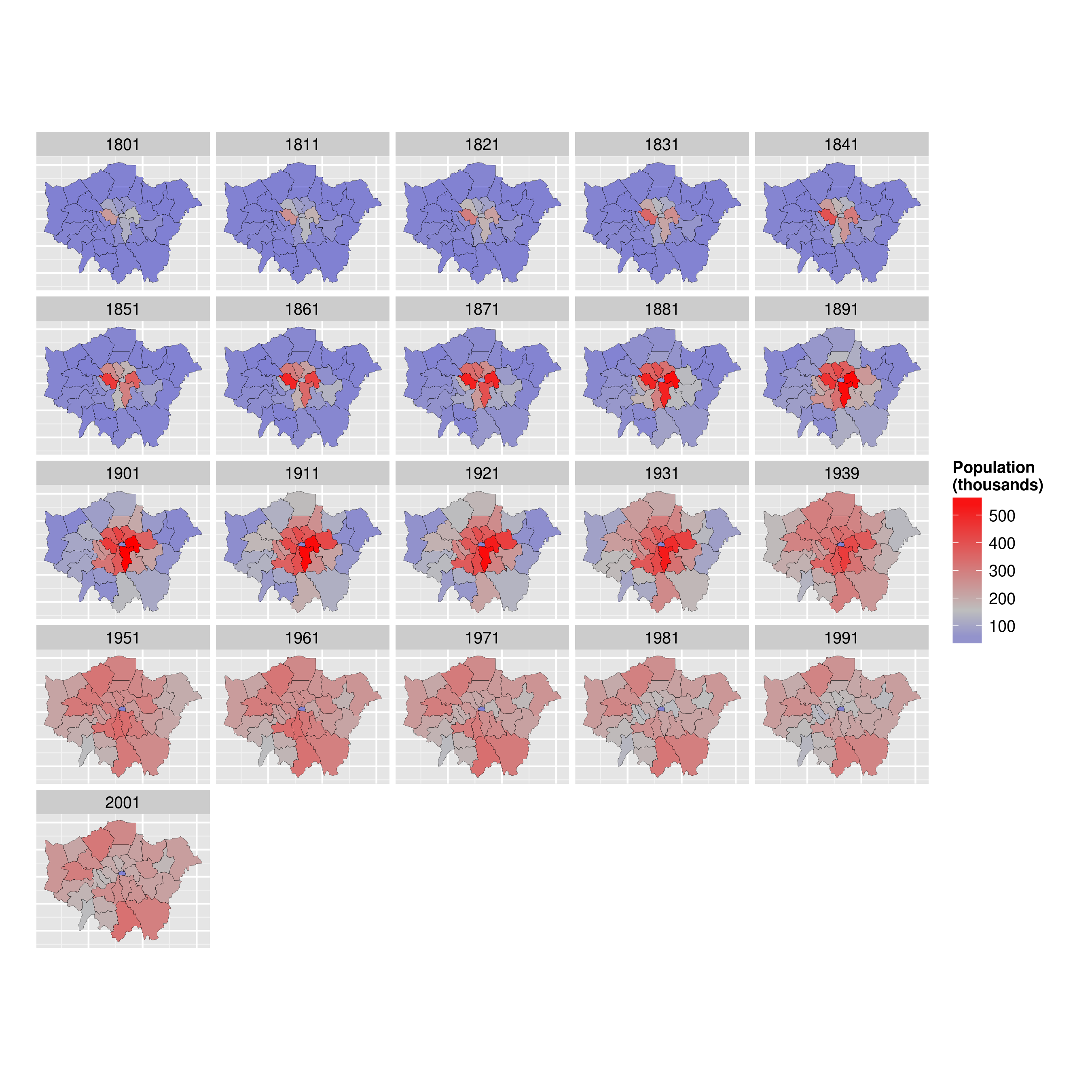
By the end of the tutorial you should have the confidence and skills needed to convert a diverse range of geographical and non-geographical datasets into meaningful analyses and visualisations. Using data and code provided in this repository all of the results are reproducible, culminating in publication-quality maps such as the faceted map of London's population below:
The course will even show you how to make your maps animated:
An up-to-date pdf version of this tutorial is maintained for teaching purposes in the file
[intro-spatial-rl.pdf](https://github.com/Robinlovelace/Creating-maps-in-R/blob/master/intro-spatial-rl.pdf).
If you have any feedback on this tutorial please let us know via email or via this repository. Contibutions to the `.Rmd` file ([README.Rmd](https://github.com/Robinlovelace/Creating-maps-in-R/blob/master/README.Rmd)) are welcome. Happy mapping!
The tutorial is practical in nature: you will load-in,
visualise and manipulate spatial data.
We assume no prior knowledge of spatial data analysis but some
experience with R will help.
If you have not used R before, it may be worth following an
introductory tutorial, such as
*Efficient R Programming*
([Gillespie and Lovelace, 2016](https://csgillespie.github.io/efficientR/)), *R for Data Science* ([Grolemund and Wickham, 2016](http://r4ds.had.co.nz/)) or tutorials suggested on [rstudio.com](https://www.rstudio.com/online-learning/) and [cran.r-project.org](https://cran.r-project.org/other-docs.html).
...
Now you know some R, it's time to turn your attention towards spatial data with R. To that end, this tutorial is organised as follows:
1. Introduction: provides a guide to R's syntax and preparing for the tutorial
2. Spatial data in R: describes basic spatial functions in R
3. Creating and manipulating spatial data: includes changing projection, clipping and spatial joins
4. Map making with **tmap**, **ggplot2** and **leaflet**: this section demonstrates map
making with more advanced visualisation tools
5. Taking spatial analysis in R further: a compilation of resources for furthering your skills
To distinguish between prose and code, please be aware of the following typographic conventions used in this document: R code (e.g. `plot(x, y)`) is
written in a `monospace` font and package names (e.g. **rgdal**)
are written in **bold**.
A double hash (`##`) at the start of a line of code indicates that this is output from R. Lengthy outputs have been omitted from the document to save space, so do
not be alarmed if R produces additional messages: you can always look up them up on-line.
As with any programming language, there are often many ways to produce the same output in R. The code presented in this document is not the only way to do things. We encourage you to
play with the code to gain a deeper understanding of R.
Do not worry, you cannot 'break' anything using R and all the input data
can be re-loaded if things do go wrong. As with learning to skateboard, you learn
by falling and getting an `Error:` message in R is much less
painful than falling onto concrete! We encourage `Error:`s --- it
means you are trying new things.
Part I: Introduction
========================================================
## Prerequisites
For this tutorial you need a copy of R. The latest version
can be downloaded from [http://cran.r-project.org/](http://cran.r-project.org/).
We also suggest that you use an R editor, such as [RStudio](http://www.rstudio.com/), as this will improve the user-experience and help with the learning process. This can be downloaded from http://www.rstudio.com. The R Studio interface is comprised of a number of windows, the most important being the console window and the script window. Anything you type directly into the console window will not be saved, so use the script window to create scripts which you can save for later use. There is also a Data Environment window which lists the dataframes and objects being used. Familiarise yourself with the R Studio interface before getting started on the tutorial.
When writing code in any language, it is good practice to use consistent and clear conventions, and R is no exception.
Adding comments to your code is also useful; make these meaningful so you remember what the code is doing when you revisit it at a later date.
You can add a comment by using the `#` symbol before or after a line of code, as illustrated in the block of code below. This code should create Figure 1 if typed correctly into the Console window:
```{r fig.cap="Basic plot of x and y (right) and code used to generate the plot (right).", echo=FALSE, fig.width=6, fig.height=3}
# # Generate data
# x <- 1:400
# y <- sin(x / 10) * exp(x * -0.01)
#
# plot(x, y) # plot the result
library(png)
library(grid)
grid.raster(readPNG("figure/plot1.png"))
```
This first line in this block of code creates a new *object* called `x` and assigns it to a range of integers between 1 and 400. The second line creates another object called `y` which is assigned to a mathematical formula, and the third line plots the two together to create the plot shown.
Note `<-`, the directional "arrow" assignment symbol which creates a new object and assigns it to the value you have given.^[Tip: typing `Alt -` on the keyboard will create the arrow in RStudio.
The equals sign `=` also works.]
If you require help on any function, use the `help` command,
e.g. `help(plot)`. Because R users love being concise,
this can also be written as `?plot`. Feel free to use it
at any point you would like more detail on a specific function
(although R's help files are famously cryptic for the un-initiated).
Help on more general terms can be found using the `??` symbol. To test this,
try typing `??regression`.
For the most part, *learning by doing* is a good motto, so let's crack
on and download some packages and data.
## R Packages
R has a huge and growing number of spatial data packages. We recommend taking a quick browse on R's main website to see the spatial packages available:
[http://cran.r-project.org/web/views/Spatial.html](http://cran.r-project.org/web/views/Spatial.html).
In this tutorial we will use the packages from the '**sp**verse', that use the **sp** package:
- **ggmap**: extends the plotting package **ggplot2** for maps
- **rgdal**: R's interface to the popular C/C++ spatial data processing library [gdal](http://www.gdal.org/)
- **rgeos**: R's interface to the powerful vector processing library [geos](http://trac.osgeo.org/geos/)
- **maptools**: provides various mapping functions
- [**dplyr**](http://cran.r-project.org/web/packages/dplyr/index.html) and [**tidyr**](http://blog.rstudio.org/2014/07/22/introducing-tidyr/): fast and concise data manipulation packages
- **tmap**: a new packages for rapidly creating beautiful maps
For a tutorial based on the recent [**sf**](https://github.com/edzer/sfr) package you will have to look elsewhere, like the [geocompr](https://bookdown.org/robinlovelace/geocompr/) website, the online home of the forthcoming book *Geocomputation with R*.
Some packages may already be installed on your computer. To test if a package is installed, try to load it using the `library` function; for example, to test if **ggplot2** is installed, type `library(ggplot2)` into the console window.
If there is no output from R, this is good news: it means that the library
has already been installed on your computer.
If you get an error message,you will need to install the package using
`install.packages("ggplot2")`. The package will download from the Comprehensive R Archive Network (CRAN); if you are prompted
to select a 'mirror', select one that is close to current location.
If you have not done so already, install these packages on your computer now.
A [quick way](http://stackoverflow.com/questions/8175912/load-multiple-packages-at-once) to do this in one go is to enter the following lines of code:
```{r, eval=FALSE}
x <- c("ggmap", "rgdal", "rgeos", "maptools", "dplyr", "tidyr", "tmap")
# install.packages(x) # warning: uncommenting this may take a number of minutes
lapply(x, library, character.only = TRUE) # load the required packages
```
\clearpage
# Part II: Spatial data in R
## Starting the tutorial and downloading the data
Now that we have looked at R's basic syntax and installed the
necessary packages,let's load some real spatial data.
The next part of the tutorial will focus on plotting and interrogating
spatial objects.
```{r, echo=FALSE}
# TODO: add info about accessing online data from R
```
The data used for this tutorial can be downloaded from:
[https://github.com/Robinlovelace/Creating-maps-in-R](https://github.com/Robinlovelace/Creating-maps-in-R).
Click on the "Download ZIP" button on the right hand side of the screen and once downloaded, unzip this to a new folder on your computer.
Open the existing 'Creating-maps-in-R' project using `File -> Open File...` on the top menu.
Alternatively, use the *project menu* to open the project or create a new one. It is *highly recommended* that you use RStudio's projects to organise your
R work and that you organise your files into sub-folders (e.g. `code`, `input-data`, `figures`) to avoid digital clutter (Figure 2). The RStudio website contains an overview of the
software: [rstudio.com/products/rstudio/](http://www.rstudio.com/products/rstudio/).
```{r, fig.cap="The RStudio environment with the project tab poised to open the Creating-maps-in-R project.", echo=FALSE}
grid.raster(readPNG("figure/rstudio-proj.png"))
```
Opening a project sets the current working directory to the project's parent folder, the `Creating-maps-in-R` folder in this case. If you ever need to change your working directory, you can use the 'Session' menu at the top of the page or use the [`setwd` command](http://www.statmethods.net/interface/workspace.html).
```{r, eval= F, echo=FALSE}
# Use the `setwd` command to set the working directory to the folder where the data is saved.
# If your username is "username" and you saved the files into a
# folder called "Creating-maps-in-R-master" on your Desktop, for example,
# you would type the following:
# setwd("C:/Users/username/Desktop/Creating-maps-in-R-master/")
```
The first file we are going to load into R Studio is the "london_sport" [shapefile](http://en.wikipedia.org/wiki/Shapefile) located in the 'data' folder of the project. It is worth looking at this input dataset in your file browser before opening it in R. You will notice that there are several files named "london_sport", all with different file extensions. This is because a shapefile is actually made up of a number of different files, such as .prj, .dbf and .shp.
You could also try opening the file "london_sport.shp" file in a conventional GIS such as QGIS to see what a shapefile contains.
You should also open "london_sport.dbf" in a spreadsheet program such as
LibreOffice Calc. to see what this file contains. Once you think you understand the input data, it's time to open it in R. There are a number of ways to do this,
the most commonly used and versatile of which is `readOGR`.
This function, from the **rgdal** package, automatically extracts the information regarding the data.
**rgdal** is R’s interface to the "Geospatial Abstraction Library (GDAL)"
which is used by other open source GIS packages such as QGIS and enables
R to handle a broader range of spatial data formats. If you've not already
*installed* and loaded the **rgdal** package (see the 'prerequisites and packages' section) do so now:
```{r, message=FALSE, results='hide'}
library(rgdal)
lnd <- readOGR(dsn = "data/london_sport.shp")
# lnd <- readOGR(dsn = "data", layer = "london_sport")
```
In the second line of code above the `readOGR` function is used to load a shapefile and assign it to a new spatial object called `lnd`, short for London.
`readOGR` is a *function* of the **rgdal** package, the first *argument* of which `dsn`: "data source name", the file or directory of the geographic data to be loaded.
Thanks to recent developments in **rgdal**, the layer no longer has to be specified (as it is in the 3 line of code which has been *commented
out*).^[The
third line of code is included for historical interest and to provide an opportunity to discuss R functions and their arguments (the values inside a function's brackets) in detail. Note the arguments are separated by a comma. The order in which they are specified is important. You do not have to explicitly type `dsn =` or `layer =` as R knows which order they appear. `readOGR("data", "london_sport")` would work just as well. For clarity, it is good practice to include argument names when learning new functions so we will continue to do so.
]
`lnd` is now an object representing the population of London Boroughs in 2001 and the percentage of the population participating in sporting activities according to the
[Active People Survey](http://data.london.gov.uk/datastore/package/active-people-survey-kpi-data-borough).
The boundary data is from the [Ordnance Survey](http://www.ordnancesurvey.co.uk/oswebsite/opendata/).
For information about how to load different types of spatial data,
see the help documentation for `readOGR`. This can be accessed by typing `?readOGR`.
For another worked example, in which a GPS trace is loaded,
please see Cheshire and Lovelace (2014).
## The structure of spatial data in R
Spatial objects like the `lnd` object are made up of a number of different *slots*, the key *slots* being `@data` (non geographic *attribute data*) and `@polygons` (or `@lines` for line data). The data *slot* can be thought of as an attribute table and the geometry *slot* is the polygons that make up the physcial boundaries. Specific *slots*
are accessed using the `@` symbol. Let's now analyse the sport object with some basic commands:
```{r}
head(lnd@data, n = 2)
mean(lnd$Partic_Per) # short for mean(lnd@data$Partic_Per)
```
Take a look at the output created (note the table format of the data and the column names). There are two important symbols at work in the above block of code: the `@` symbol in the first line of code is used to refer to the data *slot* of the `lnd` object. The `$` symbol refers to the `Partic_Per` column (a variable within the table) in the `data` *slot*, which was identified from the result of running the first line of code.
The `head` function in the first line of the code above simply means "show the first few lines of data" (try entering `head(lnd@data)`, see `?head` for more details).
The second line calculates finds the mean sports participation per 100 people for zones in London.
The results works because we are dealing with numeric data.
To check the classes of all the variables in a spatial dataset, you can use the following command:
```{r}
sapply(lnd@data, class)
```
This shows that, unexpectedly, `Pop_2001` is a factor. We can *coerce* the variable into the correct, numeric, format with the following command:
```{r}
lnd$Pop_2001 <- as.numeric(as.character(lnd$Pop_2001))
```
Type the function again but this time hit `tab` before completing the command. RStudio has auto-complete functionality which can save you a lot of time in the long run (see Figure 3).
```{r, fig.height=1.3, echo=FALSE, fig.cap="Tab-autocompletion in action: display from RStudio after typing `lnd@` then `tab` to see which slots are in `lnd`"}
grid.raster(readPNG("figure/tab-complete.png"))
```
To explore `lnd` object further, try typing `nrow(lnd)` (display number of rows) and record how many zones the dataset contains. You can also try `ncol(lnd)`.
One issue with the data that we have loaded is that it has no coordinate reference system (CRS):
```{r}
lnd@proj4string
```
## Basic plotting
Now we have seen something of the structure of spatial objects in R,
let us look at plotting them. Note, that plots
use the *geometry* data, contained primarily in the `@polygons` slot.
```{r, eval=FALSE}
plot(lnd) # not shown in tutorial - try it on your computer
```
`plot` is one of the most useful functions in R, as it changes its behaviour
depending on the input data (this is called *polymorphism* by computer scientists).
Inputting another object such as `plot(lnd@data)` will generate
an entirely different type of plot. Thus R is intelligent at guessing what you want to do with the data you provide it with.
R has powerful subsetting capabilities that can be accessed very concisely using square brackets,as shown in the following example:
```{r}
# select rows of lnd@data where sports participation is less than 13
lnd@data[lnd$Partic_Per < 13, 1:3]
```
The above line of code asked R to select only the rows from the `lnd` object, where sports participation is lower than 13,
in this case rows 17, 21 and 32, which are Harrow, Newham and the city centre respectively. The square brackets work as follows:
anything before the comma refers to the rows that will be selected, anything after
the comma refers to the number of columns that should be returned.
For example if the data frame had 1000 columns and you were only interested in the first two columns you could specify `1:2` after the comma. The ":" symbol simply means "to", i.e. columns 1 to 2. Try experimenting with the square brackets notation
(e.g. guess the result of `lnd@data[1:2, 1:3]` and test it).
So far we have been interrogating only the attribute data *slot* (`@data`) of the `lnd` object, but the square brackets can also be used to subset spatial objects, i.e. the geometry *slot*. Using the same logic as before try
to plot a subset of zones with high sports participation.
```{r, eval=FALSE}
# Select zones where sports participation is between 20 and 25%
sel <- lnd$Partic_Per > 20 & lnd$Partic_Per < 25
plot(lnd[sel, ]) # output not shown here
head(sel) # test output of previous selection (not shown)
```
This plot is quite useful, but it only displays the areas which meet the criteria. To see the sporty areas in context with the other areas of the map simply use the `add = TRUE` argument after the initial plot.
(`add = T` would also work, but we like to spell things out in this tutorial for clarity).
What do you think the `col` argument refers to in the below block? (see Figure 5).
If you wish to experiment with multiple criteria queries, use `&`.
```{r fig.cap="Simple plot of London with areas of high sports participation highlighted in blue"}
plot(lnd, col = "lightgrey") # plot the london_sport object
sel <- lnd$Partic_Per > 25
plot(lnd[ sel, ], col = "turquoise", add = TRUE) # add selected zones to map
```
Congratulations! You have just interrogated and visualised a
spatial object: where are areas with high levels of sports
participation in London? The map tells us. Do not worry for now about
the intricacies of
how this was achieved: you have learned vital basics of how R works as a language;
we will cover this in more detail in subsequent sections.
As a bonus stage, select and plot
only zones that are
close to the centre of London (see Figure 5). Programming encourages rigorous
thinking and it helps to define the problem
more specifically:
> **Challenge**: Select all zones whose geographic centroid lies within 10 km of the geographic centroid of inner
London.^[To
see how this map was created, see the code
in [README.Rmd](https://github.com/Robinlovelace/Creating-maps-in-R/blob/master/README.Rmd) . This may be loaded by typing
`file.edit("README.Rmd")` or online at [github.com/Robinlovelace/Creating-maps-in-R/blob/master/README.Rmd](https://github.com/Robinlovelace/Creating-maps-in-R/blob/master/README.Rmd).]
```{r, echo=FALSE, fig.cap="Zones in London whose centroid lie within 10 km of the geographic centroid of the City of London. Note the distinction between zones which only touch or 'intersect' with the buffer (light blue) and zones whose centroid is within the buffer (darker blue).", message=FALSE}
library(rgeos)
plot(lnd, col = "grey")
# find London's geographic centroid (add ", byid = T" for all)
cent_lnd <- gCentroid(lnd[lnd$name == "City of London",])
points(cent_lnd, cex = 3)
# set 10 km buffer
lnd_buffer <- gBuffer(spgeom = cent_lnd, width = 10000)
# method 1 of subsetting selects any intersecting zones
lnd_central <- lnd[lnd_buffer,] # the selection is too big!
# test the selection for the previous method - uncomment below
plot(lnd_central, col = "lightblue", add = T)
plot(lnd_buffer, add = T) # some areas just touch the buffer
# method2 of subsetting selects only points within the buffer
lnd_cents <- SpatialPoints(coordinates(lnd),
proj4string = CRS(proj4string(lnd))) # create spatialpoints
sel <- lnd_cents[lnd_buffer,] # select points inside buffer
points(sel) # show where the points are located
lnd_central <- lnd[sel,] # select zones intersecting w. sel
plot(lnd_central, add = T, col = "lightslateblue",
border = "grey")
plot(lnd_buffer, add = T, border = "red", lwd = 2)
# Add text to the plot!
text(coordinates(cent_lnd), "Central\nLondon")
```
## Selecting quadrants
The code below should help understand the way spatial data work in R.
```{r}
# Find the centre of the london area
easting_lnd <- coordinates(gCentroid(lnd))[[1]]
northing_lnd <- coordinates(gCentroid(lnd))[[2]]
# arguments to test whether or not a coordinate is east or north of the centre
east <- sapply(coordinates(lnd)[,1], function(x) x > easting_lnd)
north <- sapply(coordinates(lnd)[,2], function(x) x > northing_lnd)
# test if the coordinate is east and north of the centre
lnd$quadrant <- "unknown" # prevent NAs in result
lnd$quadrant[east & north] <- "northeast"
```
> **Challenge**: Based on the the above code as refrence try and find the remaining 3 quadrants and colour them as per Figure 6.
Hint - you can use the **llgridlines** function in order to overlay the long-lat lines.
For bonus points try to desolve the quadrants so the map is left with only 4 polygons.
```{r, echo=FALSE, fig.cap="The 4 quadrants of London and dissolved borders. Challenge: recreate a plot that looks like this.", fig.show='hold', out.height="5cm"}
lnd$quadrant[!east & north] <- "northwest"
lnd$quadrant[east & !north] <- "southeast"
lnd$quadrant[!east & !north] <- "southwest"
plot(lnd)
plot(lnd[east & north,], add = TRUE, col = "red" )
llgridlines(lnd, lty= 3, side ="EN", offset = -0.5)
lnd_disolved = rgeos::gUnaryUnion(spgeom = lnd, id = lnd$quadrant)
library(tmap)
qtm(lnd, fill = "quadrant") +
tm_shape(lnd_disolved) +
tm_borders(lwd = 9)
```
\clearpage
# Part III: Creating and manipulating spatial data
```{r, echo=FALSE}
# should be manipulating and plotting. TODO: talk about base graphics
```
Alongside visualisation and interrogation, a GIS must also
be able to create and modify spatial data. R's spatial packages
provide a very wide and powerful suite of
functionality for processing and creating spatial data.
*Reprojecting* and *joining/clipping*
are fundamental GIS operations, so in this section we will explore how these operations can be undertaken in R. Firstly We will join non-spatial data to spatial data so it can be mapped.
Finally we will cover spatial joins, whereby
information from two spatial objects is
combined based on spatial location.
## Creating new spatial data
R objects can be created by entering the name of the
class we want to make. `vector` and `data.frame`
objects for example, can be
created as follows:
```{r}
vec <- vector(mode = "numeric", length = 3)
df <- data.frame(x = 1:3, y = c(1/2, 2/3, 3/4))
```
We can check the class of these new objects using `class()`:
```{r}
class(vec)
class(df)
```
The same logic applies to spatial data. The input must be a numeric matrix or data.frame:
```{r}
sp1 <- SpatialPoints(coords = df)
```
We have just created a spatial points object,
one of the fundamental data
types for spatial data. (The others are lines, polygons
and pixels, which can be created by `SpatialLines`,
`SpatialPolygons` and `SpatialPixels`, respectively.)
Each type of spatial data has a corollary that can accepts
non-spatial data, created by adding `DataFrame`.
`SpatialPointsDataFrame()`, for example, creates points
with an associated `data.frame`. The number of rows
in this dataset must equal the number of features in the
spatial object, which in the case of `sp1` is 3.
```{r}
class(sp1)
spdf <- SpatialPointsDataFrame(sp1, data = df)
class(spdf)
```
The above code extends the pre-existing object `sp1` by adding
data from `df`. To see how strict spatial classes are,
try replacing `df` with `mat` in the above code: it causes an error. All spatial data classes can be created in a similar way,
although `SpatialLines` and `SpatialPolygons` are much more
complicated (Bivand et al. 2013). More frequently your spatial
data will be read-in from an externally-created file, e.g.
using `readOGR()`. Unlike the spatial objects we created above,
most spatial data comes with an associate 'CRS'.
## Projections: setting and transforming CRS in R
The *Coordinate Reference System* (CRS) of spatial objects
defines where they are placed on the Earth's surface.
You may have noticed '`proj4string` 'in the
summary of `lnd` above:
the information that follows represents its CRS.
Spatial data should always have a CRS.
If no CRS information is provided, and the correct CRS is known,
it can be set as follow:
```{r, warning=FALSE}
proj4string(lnd) <- NA_character_ # remove CRS information from lnd
proj4string(lnd) <- CRS("+init=epsg:27700") # assign a new CRS
```
R issues a warning when the CRS is changed. This is so the user
knows that they are simply changing the CRS, not *reprojecting* the data.
An easy way to refer to different projections
is via [EPSG codes](http://www.epsg-registry.org/).
Under this system `27700` represents the British National Grid.
'WGS84' (`epsg:4326`) is a very commonly used CRS worldwide.
The following code shows how to search the list of available EPSG
codes and create a new version of `lnd` in WGS84:^[Note:
entering `projInfo()` provides additional CRS options. [spatialreference.org](http://spatialreference.org/)
provides more information about EPSG codes.]
```{r}
EPSG <- make_EPSG() # create data frame of available EPSG codes
EPSG[grepl("WGS 84$", EPSG$note), ] # search for WGS 84 code
lnd84 <- spTransform(lnd, CRS("+init=epsg:4326")) # reproject
```
Above, `spTransform` converts the coordinates of
`lnd` into the widely used WGS84 CRS.
Now we've transformed `lnd` into
a more widely used CRS,
it is worth saving it. R stores data efficiently in
`.RData` or `.Rds` formats.
The former is more restrictive and maintains the object's
name, so we use the latter.
```{r}
# Save lnd84 object (we will use it in Part IV)
saveRDS(object = lnd84, file = "data/lnd84.Rds")
```
Now we can remove the `lnd84` object with the `rm` command. It will be useful
later. (In RStudio, notice it also disappears from the Environment in the top
right panel.)
```{r}
rm(lnd84) # remove the lnd object
# we will load it back in later with readRDS(file = "data/lnd84.Rds")
```
## Attribute joins
Attribute joins are used to link additional pieces of information to our polygons.
In the `lnd` object, for example, we have 4 attribute variables --- that can be
found by typing `names(lnd)`. But what happens when we want to add more
variables from an external source? We will use the example of recorded crimes by
London boroughs to demonstrate this.
To reaffirm our starting point, let's re-load the
"london_sport" shapefile as a new object and plot it:
```{r, eval=FALSE}
library(rgdal) # ensure rgdal is loaded
# Create new object called "lnd" from "london_sport" shapefile
lnd <- readOGR("data/london_sport.shp")
plot(lnd) # plot the lnd object (not shown)
nrow(lnd) # return the number of rows (not shown)
```
```{r, eval=FALSE, echo=FALSE}
## Downloading additional data
# Because we are using borough-level data, and boroughs are official administrative
# zones, there is much data available at this level. We will use the example
# of crime data to illustrate this data availability, and join this with the current
# spatial dataset. As before, we can download and import the data from within R:
# download.file("http://data.london.gov.uk/datafiles/crime-community-safety/mps-
# recordedcrime-borough.csv", destfile = "mps-recordedcrime-borough.csv")
# uncomment and join the above code to download the data
crime_data <- read.csv("data/mps-recordedcrime-borough.csv",
stringsAsFactors = FALSE)
head(crime_data)
# Initially, the `read.csv` may an error. If not the `head` command should show
# that the dataset has not loaded correctly. This was due to an unusual
# encoding used in the text file: hopefully you will not
# encounter this problem in your research, but it highlights the importance
# of checking the input data. To overcome this issue we
# can set the encoding manually, and continue.
# variant: markdown_github
```
The non-spatial data we are going to join to the `lnd` object
contains records of crimes in London. This is stored in a comma separated values
[(`.csv`)](https://raw.githubusercontent.com/Robinlovelace/Creating-maps-in-R/master/data/mps-recordedcrime-borough.csv) file called "mps-recordedcrime-borough".
If you open the [file](https://raw.githubusercontent.com/Robinlovelace/Creating-maps-in-R/master/data/mps-recordedcrime-borough.csv)
in a separate spreadsheet application first, we can see each row represents a single reported crime.
We are going to use a function called `aggregate`
to aggregate the crimes at the borough level, ready to join to our spatial
`lnd` dataset. A new object called `crime_data` is created to store this data.
```{r, echo=FALSE, eval=FALSE}
# # convert crime_data and rename cols
# crime_data <- read.csv("data/mps-recordedcrime-borough.csv",
# fileEncoding = "UCS-2LE")
# names(crime_data)
# crime_data <- rename(crime_data, DName = Spatial_DistrictName)
# write.csv(crime_data, file = "data/mps-recordedcrime-borough.csv")
```
```{r, results='hide'}
# Create and look at new crime_data object
crime_data <- read.csv("data/mps-recordedcrime-borough.csv",
stringsAsFactors = FALSE)
head(crime_data$CrimeType) # information about crime type
# Extract "Theft & Handling" crimes and save
crime_theft <- crime_data[crime_data$CrimeType == "Theft & Handling", ]
head(crime_theft, 2) # take a look at the result (replace 2 with 10 to see more rows)
# Calculate the sum of the crime count for each district, save result
crime_ag <- aggregate(CrimeCount ~ Borough, FUN = sum, data = crime_theft)
# Show the first two rows of the aggregated crime data
head(crime_ag, 2)
```
You should not expect to understand all of this upon first try: simply typing the commands and thinking briefly about the outputs is all that is needed at this stage. Here are a few things that you may not have seen before that will likely be useful in the future:
- In the first line of code when we read in the file we specify its location (check in your
file browser to be sure).
- The `==` function is used to select only those observations that
meet a specific condition i.e. where it is equal to, in this case all crimes involving "Theft and Handling".
- The
`~` symbol means "by": we aggregated the `CrimeCount` variable by the district name.
Now that we have crime data at the borough level, the challenge is to join it to the `lnd` object. We will base our join on the `Borough` variable from the `crime_ag` object and the `name` variable from the `lnd` object. It is not always straight-forward to join objects based on names as the names do not always match. Let's see which names in the `crime_ag` object match the spatial data object, `lnd`:
```{r}
# Compare the name column in lnd to Borough column in crime_ag to see which rows match.
lnd$name %in% crime_ag$Borough
# Return rows which do not match
lnd$name[!lnd$name %in% crime_ag$Borough]
```
The first line of code above uses the `%in%` command to
identify which values in `lnd$name` are also contained in the Borough names of the
aggregated crime data. The results indicate that all but one of the borough names matches.
The second line of code tells us that it is 'City of London'. This does not exist in the
crime data. This may be because the City of London has it's own Police
Force.^[See [www.cityoflondon.police.uk/](https://www.cityoflondon.police.uk/).]
(The borough name in the crime data does not
match `lnd$name` is 'NULL'. Check this by typing
`crime_ag$Borough[!crime_ag$Borough %in% lnd$name]`.)
> **Challenge:** identify the number of
crimes taking place in borough 'NULL', less than
4,000.
Having checked the data found that one
borough does not match, we are now ready to join the spatial and non-spatial datasets. It is recommended to use
the `left_join` function from the **dplyr** package but the `merge` function
could equally be used. Note that when we ask for help for a function
that is not loaded, nothing happens, indicating we need to load it:
```{r, results='hide', eval=FALSE}
library(dplyr) # load dplyr
```
We use `left_join` because we want the length of the data frame
to remain unchanged, with variables from new data appended in
new columns (see `?left_join`).
The `*join` commands (including `inner_join` and `anti_join`) assume, by default, that matching variables have the same name.
Here we will specify the association between variables in the two data sets:
```{r, echo=FALSE, message=FALSE}
# Load dplyr package
library(dplyr)
```
```{r, results='hide'}
head(lnd$name) # dataset to add to (results not shown)
head(crime_ag$Borough) # the variables to join
# head(left_join(lnd@data, crime_ag)) # test it works
lnd@data <- left_join(lnd@data, crime_ag, by = c('name' = 'Borough'))
```
Take a look at the new `lnd@data` object. You should
see new variables added, meaning the attribute join
was successful. Congratulations! You
can now plot the rate of theft crimes in London by borough (see Fig 8).
```{r, eval=FALSE}
library(tmap) # load tmap package (see Section IV)
qtm(lnd, "CrimeCount") # plot the basic map
```
```{r, echo=FALSE, eval=FALSE}
# This is the modified version of the code, to create the map displayed
library(tmap)
library(tmaptools)
lnd_wgs = spTransform(lnd, CRS("+init=epsg:4326"))
osm_tiles = read_osm(bbox(lnd_wgs))
lnd_wgs$Thefts <- lnd$CrimeCount / 10000
tm_shape(osm_tiles) +
tm_raster() +
tm_shape(lnd_wgs) +
tm_fill("Thefts", fill.title = "Thefts\n(10000)", scale = 0.8, alpha = 0.5) +
tm_layout(legend.position = c(0.89,0.02))
```
```{r, echo=FALSE, fig.cap="Number of thefts per borough.", out.width="48%", fig.align="center"}
grid.raster(readPNG("figure/lnd-crime.png"))
```
> **Optional challenge:** create a map of additional variables in London
With the attribute joining skills you have learned in this section,
you should now be able to take datasets from many sources, e.g. [data.london.gov.uk](http://data.london.gov.uk/dataset/london-borough-profiles), and
join them to your geographical data.
## Clipping and spatial joins
In addition to joining by attribute (e.g. Borough
name), it is also possible to do
[spatial joins](http://help.arcgis.com/en/arcgisdesktop/10.0/help/index.html#//00080000000q000000)
in R. We use transport infrastructure points as the spatial data to join,
with the aim of finding out about how many are found in each London borough.
```{r, results='hide'}
library(rgdal)
# create new stations object using the "lnd-stns" shapefile.
stations <- readOGR(dsn = "data/lnd-stns.shp")
# stations = read_shape("data/lnd-stns.shp") # from tmap
proj4string(stations) # this is the full geographical detail.
proj4string(lnd) # what's the coordinate reference system (CRS)
bbox(stations) # the extent, 'bounding box' of stations
bbox(lnd) # return the bounding box of the lnd object
```
The `proj4string()` function shows that the Coordinate Reference System (CRS)
of `stations` differs from that of our `lnd` object.
OSGB 1936 (or [EPSG 27700](http://spatialreference.org/ref/epsg/27700/))
is the official CRS for the UK, so
we will convert the 'stations' object to this:
```{r fig.cap="Sampling and plotting stations"}
# Create reprojected stations object
stations <- spTransform(stations, CRSobj = CRS(proj4string(lnd)))
plot(lnd) # plot London
points(stations) # overlay the station points
```
Note the `stations` points now overlay the boroughs but that
the spatial extent of `stations` is
greater than that of `lnd`.
To clip the `stations`
so that only those falling within London boroughs are retained we can use
`sp::over`, or simply the square bracket notation for subsetting tabular data
(enter `?gIntersects` to find out another way to do this):
```{r fig.cap="The clipped stations dataset"}
stations <- stations[lnd, ]
plot(stations) # test the clip succeeded
```
```{r, echo=F,eval=FALSE}
# save(lnd, file="data/lnd.RData")
# save(stations, file="data/stations.RData")
```
`gIntersects` can achieve the same result, but with more lines of code
(see [www.rpubs.com/RobinLovelace](http://www.rpubs.com/RobinLovelace/11796) for more on this) .
\clearpage
# Part IV: Making maps with tmap, ggplot2 and leaflet
## **tmap**
[**tmap**](https://github.com/mtennekes/tmap)
was created
to overcome some of the limitations of base graphics
and **ggmap**. A concise introduction to
**tmap** can be accessed (after the package is installed)
by using the vignette function:
```{r, eval=FALSE}
# install.packages("tmap") # install the CRAN version
library(tmap)
vignette("tmap-nutshell")
```
```{r, echo=FALSE, message=FALSE}
library(tmap)
```
A couple of basic plots show the package's intuitive
syntax and attractive default parameters.
```{r, eval=FALSE, message=FALSE}
qtm(shp = lnd, fill = "Partic_Per", fill.palette = "-Blues") # not shown
```
```{r, fig.cap="Side-by-side maps of sports participation and population"}
qtm(shp = lnd, fill = c("Partic_Per", "Pop_2001"), fill.palette = "Blues", ncol = 2)
```
The plot above shows the ease with which tmap can create maps
next to each other for different variables. The plot produced by the following code chunk (not shown) demonstrates
the power of the `tm_facets` command. Note that all the maps created with the `qtm` function can also be created with `tm_shape`, followed by `tm_fill` (or another `tm_` function).
```{r, fig.cap="Facetted map of London Boroughs created by tmap", eval=FALSE}
tm_shape(lnd) +
tm_fill("Pop_2001", thres.poly = 0) +
tm_facets("name", free.coords = TRUE, drop.units = TRUE)
```
To create a basemap with tmap, you can use the `read_osm` function, from the [**tmaptools** package](https://github.com/mtennekes/tmaptools) as follows. Note that you must first transform the data into a *geographical* CRS:
```{r, fig.cap="London's population in 2001.", fig.width=4}
# Transform the coordinate reference system
lnd_wgs = spTransform(lnd, CRS("+init=epsg:4326"))
if(curl::has_internet()) {
osm_tiles = tmaptools::read_osm(bbox(lnd_wgs)) # download images from OSM
tm_shape(osm_tiles) + tm_raster() +
tm_shape(lnd_wgs) +
tm_fill("Pop_2001", fill.title = "Population, 2001", scale = 0.8, alpha = 0.5) +
tm_layout(legend.position = c(0.89, 0.02))
} else {
tm_shape(lnd_wgs) +
tm_fill("Pop_2001", fill.title = "Population, 2001", scale = 0.8, alpha = 0.5) +
tm_layout(legend.position = c(0.89, 0.02))
}
```
Another way to make **tmap** maps have a basemap is by entering `tmap_mode("view")`. This will make the maps appear on a zoomable webmap powered by **leaflet**.
There are many other intuitive and powerful functions in **tmap**. Check the documentation to find out more:
```{r, eval=FALSE}
?tmap # get more info on tmap
```
## **ggmap**
**ggmap** is based on the **ggplot2** package,
an implementation of the Grammar of Graphics (Wilkinson 2005).
**ggplot2** can replace
the base graphics in R (the functions you have been plotting with so far).
It contains default options that match good visualisation practice
and is well-documented:
http://docs.ggplot2.org/current/ .
As a first attempt with **ggplot2** we can create a scatter plot with the attribute data in the `lnd` object created previously:
```{r}
library(ggplot2)
p <- ggplot(lnd@data, aes(Partic_Per, Pop_2001))
```
The real power of **ggplot2** lies in its ability to add layers to a plot. In this case we can add text to the plot.
```{r fig.cap="ggplot for text", fig.height=3, fig.width=4}
p + geom_point(aes(colour = Partic_Per, size = Pop_2001)) +
geom_text(size = 2, aes(label = name))
```
This idea of layers (or geoms) is quite different from the standard plot functions in R, but you will find that each of the functions does a lot of clever stuff to make plotting much easier (see the documentation for a full list).
In the following steps we will create a map to show the percentage of the population in each London Borough who regularly participate in sports activities.
**ggmap** requires spatial data to be supplied as `data.frame`, using `tidy()`. The generic plot() function can use `Spatial*` objects directly; **ggplot2** cannot. Therefore we need to extract them as a data frame. The `tidy` function was written specifically for this purpose. For this to work, **broom** package must be installed.
```{r}
lnd_f <- broom::tidy(lnd)
```
This step has lost the attribute information associated with the lnd object. We can add it back using the `left_join`
function from the **dplyr** package
(see `?left_join`).
```{r, results='hide'}
head(lnd_f, n = 2) # peak at the fortified data
lnd$id <- row.names(lnd) # allocate an id variable to the sp data
head(lnd@data, n = 2) # final check before join (requires shared variable name)
lnd_f <- left_join(lnd_f, lnd@data) # join the data
```
The new`lnd_f` object contains coordinates alongside the attribute information associated with each London Borough.
It is now straightforward to produce a map with
**ggplot2**.
`coord_equal()` is the equivalent of `asp = T` in regular plots with R:
```{r fig.cap="Map of Lond Sports Participation"}
map <- ggplot(lnd_f, aes(long, lat, group = group, fill = Partic_Per)) +
geom_polygon() + coord_equal() +
labs(x = "Easting (m)", y = "Northing (m)",
fill = "% Sports\nParticipation") +
ggtitle("London Sports Participation")
```
Entering `map` should result in your first ggplot-made map of London.
The default colours are really nice but we may wish to produce the map in black and white,
which should produce a map like the one shown below. Try changing the colours and saving plots with `ggsave()`.
```{r fig.cap="Greyscale map"}
map + scale_fill_gradient(low = "white", high = "black")
```
## Creating interactive maps with **leaflet**
[Leaflet](http://leafletjs.com/) is the world's premier web
mapping system, serving hundreds of thousands of maps worldwide each day.
The JavaScript library actively developed at
[github.com/Leaflet/Leaflet](https://github.com/Leaflet/Leaflet),
has a strong user community. It is fast, powerful and easy to learn.
The **leaflet** package
creates interactive web maps in few
lines of code. One of the exciting things about the package is
its tight integration with the R package for interactive on-line
visualisation, **shiny**.
Used together, these allow R to act as a complete map-serving
platform, to compete with the likes of GeoServer!
For more information on **rstudio/leaflet**, see
[rstudio.github.io/leaflet/](https://rstudio.github.io/leaflet/) and
the following on-line tutorial:
[robinlovelace.net/r/2015/02/01/leaflet-r-package.html](http://robinlovelace.net/r/2015/02/01/leaflet-r-package.html).
```{r, eval=FALSE}
install.packages("leaflet")
library(leaflet)
lnd84 <- readRDS('data/lnd84.Rds')
leaflet() %>%
addTiles() %>%
addPolygons(data = lnd84)
```
```{r, echo=FALSE, fig.cap="The lnd84 object loaded in rstudio via the leaflet package"}
grid.raster(readPNG("figure/rstudio-leaflet.png"))
```
## Advanced Task: Faceting for Maps
```{r, echo=FALSE}
# library(reshape2) # old way of doing
# If not install it, or skip the next two steps
```
The below code demonstrates how to read in the necessary data for
this task and 'tidy' it up. The data file contains historic population values between 1801 and 2001 for London, again from the London data store.
We `tidy` the data so that the columns become rows. In other words,
we convert the data from 'flat' to 'long' format, which is the form
required by **ggplot2** for faceting graphics: the date of the
population survey becomes a variable in its own right, rather than
being strung-out over many columns.
```{r, results='hide'}
london_data <- read.csv("data/census-historic-population-borough.csv")
# install.packages("tidyr")
library(tidyr) # if not install it, or skip the next two steps
ltidy <- gather(london_data, date, pop, -Area.Code, -Area.Name)
head(ltidy, 2) # check the output (not shown)
```
In the above code we take the `london_data` object and create the
column names 'date' (the date of the record, previously spread
over many columns) and 'pop' (the population which varies). The
minus (`-`) symbol in this context tells gather not to include the
`Area.Name` and `Area.Code` as columns to be removed. In other words,
"leave these columns be". Data tidying is an important subject: more can
be read on the subject in Wickham (2014) or in a `vignette` about
the package, accessed from within R by entering `vignette("tidy-data")`.
```{r, echo=FALSE, eval=FALSE}
# lnd_molten <- melt(london_data, id = c("Area.Code", "Area.Name"))
# lnd_molten <- read.csv("data/london_data_melt.csv")
# head(lnd_molten)
# names(lnd_molten)[3] <- "date"
# Only do this step if reshape and melt failed
```
Merge the population data with the London borough geometry contained within our `lnd_f` object, using the `left_join` function from
the **dplyr** package:
```{r}
head(lnd_f, 2) # identify shared variables with ltidy
ltidy <- rename(ltidy, ons_label = Area.Code) # rename Area.code variable
lnd_f <- left_join(lnd_f, ltidy)
```
```{r, echo=FALSE}
# old way of doing it
# lnd_f <- merge(lnd_f, ltidy, by.x = "id", by.y = "Area.Code")
```
Rename the date variable (use `?gsub` and Google 'regex' to find out more).
```{r}
lnd_f$date <- gsub(pattern = "Pop_", replacement = "", lnd_f$date)
```
We can now use faceting to produce one map per year:
```{r fig.cap="Faceted plot of the distribution of London's population over time", fig.height=6, fig.width=5}
ggplot(data = lnd_f, # the input data
aes(x = long, y = lat, fill = pop/1000, group = group)) + # define variables
geom_polygon() + # plot the boroughs
geom_path(colour="black", lwd=0.05) + # borough borders
coord_equal() + # fixed x and y scales
facet_wrap(~ date) + # one plot per time slice
scale_fill_gradient2(low = "blue", mid = "grey", high = "red", # colors
midpoint = 150, name = "Population\n(thousands)") + # legend options
theme(axis.text = element_blank(), # change the theme options
axis.title = element_blank(), # remove axis titles
axis.ticks = element_blank()) # remove axis ticks
# ggsave("figure/facet_london.png", width = 9, height = 9) # save figure
```
There is a lot going on here so explore the documentation to make sure you understand it.
Try out different colour values as well.
Try experimenting with the above code block to see what effects you can
produce.
> **Challenge 1:** Try creating this plot for the % of population instead of the absolute population.
> **Challenge 2:** For bonus points, try creating an animation of London's evolving population over time (hint: a file called ggnaminate.R may help).
```{r, echo=FALSE}
# **Creating an animation of population change over time**
# library(animation)
```
# Part V: Taking spatial data analysis in R further
The skills taught in this tutorial are applicable to a very wide
range of situations, spatial or not. Often experimentation is the
most rewarding learning method, rather than just searching for the
'best' way of doing something (Kabakoff, 2011).
We recommend you play around with your data.
If you enjoyed this tutorial, you may find the
book chapter "Spatial Data Visualisation with R" of interest
(Cheshire and Lovelace, 2014). The project's repository
can be found on its GitHub page:
[github.com/geocomPP/sdvwR](https://github.com/geocomPP/sdvwR).
There are also a number of bonus 'vignettes' associated with
the present tutorial. These can be found on the
[vignettes page](https://github.com/Robinlovelace/Creating-maps-in-R/tree/master/vignettes) of the project's repository.
Other advanced tutorials include
- The Simple Features vignettes.
- "solaR: Solar Radiation and Photovoltaic Systems with R", a [technical
academic paper](http://www.jstatsoft.org/v50/i09/paper)
on the solaR package which contains a number of spatial
functions.
Such tutorials are worth doing as they will help you
understand R's spatial 'ecosystem' as a cohesive whole
rather than as a collection of isolated functions.
In R the whole is greater than
the sum of its parts.
The supportive on-line communities surrounding large open source programs such as R
are one of their greatest assets, so we recommend you become an active
"[open source citizen](http://blog.cleverelephant.ca/2013/10/being-open-source-citizen.html)" rather than a passive consumer.
Good resources
that will help you further sharpen you R skills include:
* R's homepage hosts a wealth of [official](http://cran.r-project.org/manuals.html) and [contributed](http://cran.r-project.org/other-docs.html) guides.
http://cran.r-project.org
* [StackOverflow](http://stackoverflow.com/search?q=[r]) and [GIS.StackExchange](http://gis.stackexchange.com/) groups (the "[R]" search term limits the results). If your question has not been answered yet, just ask, preferably with a reproducible example.
* R's [mailing lists](http://www.r-project.org/mail.html), especially [R-sig-geo](https://stat.ethz.ch/pipermail/r-sig-geo/). See [r-project.org/mail.html](http://www.r-project.org/mail.html).
* Dorman (2014): detailed exposition of spatial data in R, with a focus on raster data. A [free sample](https://www.packtpub.com/packtlib/book/Big%20Data%20&%20Business%20Intelligence/9781783984367/4) of this book is available online.
* Bivand et al. (2013) : 'Applied spatial data analysis with R' - provides a dense and detailed overview of spatial data analysis.
# Acknowledgements
The tutorial was developed for
a series of Short Courses funded by the National Centre for Research Methods (NCRM),
via the TALISMAN node (see [geotalisman.org](http://www.geotalisman.org/)).
Thanks to the [ESRC](http://www.esrc.ac.uk/) for funding applied methods research.
Many thanks to Matt Whittle, Alistair Leak, Hannah Roberts and Phil Jones who helped develop and demonstrate
these materials. Amy O'Neill organised the course
and encouraged feedback from participants.
The final thanks is to all users and developers of open source software
for making powerful tools such as R accessible and enjoyable to use.
If you have found this tutorial useful in your work, please [cite](https://raw.githubusercontent.com/Robinlovelace/Creating-maps-in-R/master/citation.bib) it:
Lovelace, R., & Cheshire, J. (2014). Introduction to visualising spatial data in R. National Centre for Research Methods Working Papers, 14(03). Retrieved from https://github.com/Robinlovelace/Creating-maps-in-R
# References
Bivand, R. S., Pebesma, E. J., & Rubio, V. G. (2013). Applied spatial data analysis with R. Springer. 2nd ed.
Cheshire, J., & Lovelace, R. (2015). Spatial data visualisation with R. In C. Brunsdon & A. Singleton (Eds.), Geocomputation (pp. 1–14). SAGE Publications. Retrieved from https://github.com/geocomPP/sdv . Full chapter available from
https://www.researchgate.net/publication/274697165_Spatial_data_visualisation_with_R
Dorman, M. (2014). Learning R for Geospatial Analysis. Packt Publishing Ltd.
Gillespie, Colin, and Robin Lovelace. 2016. Efficient R Programming: A Practical Guide to Smarter Programming. O’Reilly Media. https://csgillespie.github.io/efficientR/.
Kabacoff, R. (2011). R in Action. Manning Publications Co.
Lamigueiro, O. P. (2012). solaR: Solar Radiation and Photovoltaic Systems with R. Journal of Statistical Software, 50(9), 1–32. Retrieved from http://www.jstatsoft.org/v50/i09
Wickham, H. (2014). Tidy data. The Journal of Statistical Software, 14(5), Retrieved from http://www.jstatsoft.org/v59/i10
Wilkinson, L. (2005). The grammar of graphics. Springer.
```{r, echo=FALSE, eval=FALSE}
system("mv README.pdf intro-spatial-rl.pdf") # change name
```