https://github.com/sigma-py/smoothfit
Smooth data fitting in N dimensions.
https://github.com/sigma-py/smoothfit
data-fitting mathematics python
Last synced: 7 months ago
JSON representation
Smooth data fitting in N dimensions.
- Host: GitHub
- URL: https://github.com/sigma-py/smoothfit
- Owner: sigma-py
- Created: 2018-04-03T13:29:18.000Z (almost 8 years ago)
- Default Branch: main
- Last Pushed: 2023-03-10T11:42:19.000Z (about 3 years ago)
- Last Synced: 2025-07-23T05:44:02.332Z (8 months ago)
- Topics: data-fitting, mathematics, python
- Homepage:
- Size: 985 KB
- Stars: 55
- Watchers: 4
- Forks: 14
- Open Issues: 5
-
Metadata Files:
- Readme: README.md
Awesome Lists containing this project
README
[](https://pypi.org/project/smoothfit)
[](https://pypi.org/pypi/smoothfit/)
[](https://github.com/nschloe/smoothfit)
[](https://pypistats.org/packages/smoothfit)
[](https://discord.gg/hnTJ5MRX2Y)
Given experimental data, it is often desirable to produce a function whose
values match the data to some degree. This package implements a robust approach
to data fitting based on the minimization problem
```math
\|\lambda\Delta f\|^2_{L^2(\Omega)} + \sum_i (f(x_i) - y_i)^2 \to\min
```
(A similar idea is used in for data smoothing in signal processing; see, e.g.,
section 8.3 in [this
document](http://eeweb.poly.edu/iselesni/lecture_notes/least_squares/least_squares_SP.pdf).)
Unlike [polynomial
regression](https://en.wikipedia.org/wiki/Polynomial_regression) or
[Gauss-Newton](https://en.wikipedia.org/wiki/Gauss%E2%80%93Newton_algorithm),
smoothfit makes no assumptions about the function other than that it is smooth.
The generality of the approach makes it suitable for function whose domain is
multidimensional, too.
### Pics or it didn't happen
#### Runge's example

[Runge's example function](https://en.wikipedia.org/wiki/Runge%27s_phenomenon) is a
tough nut for classical polynomial regression.
If there is no noise in the input data, the parameter `lmbda` can be chosen quite small
such that all data points are approximated well. Note that there are no oscillations in
the output function `u`.
```python
import matplotlib.pyplot as plt
import numpy as np
import smoothfit
a = -1.5
b = +1.5
# plot original function
x = np.linspace(a, b, 201)
plt.plot(x, 1 / (1 + 25 * x ** 2), "-", color="0.8", label="1 / (1 + 25 * x**2)")
# sample points
x0 = np.linspace(-1.0, 1.0, 21)
y0 = 1 / (1 + 25 * x0 ** 2)
plt.plot(x0, y0, "xk")
# smoothfit
basis, coeffs = smoothfit.fit1d(x0, y0, a, b, 1000, degree=1, lmbda=1.0e-6)
plt.plot(basis.mesh.p[0], coeffs[basis.nodal_dofs[0]], "-", label="smooth fit")
plt.ylim(-0.1)
plt.grid()
plt.show()
```
#### Runge's example with noise

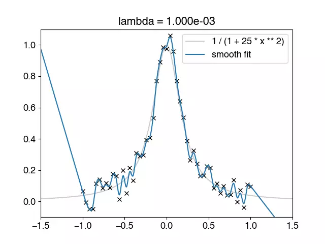
If the data is noisy, `lmbda` needs to be chosen more carefully. If too small, the
approximation tries to resolve _all_ data points, resulting in many small oscillations.
If it's chosen too large, no details are resolved, not even those of the underlying
data.
```python
import matplotlib.pyplot as plt
import numpy as np
import smoothfit
a = -1.5
b = +1.5
# plot original function
x = np.linspace(a, b, 201)
plt.plot(x, 1 / (1 + 25 * x ** 2), "-", color="0.8", label="1 / (1 + 25 * x**2)")
# 21 sample points
rng = np.random.default_rng(0)
n = 51
x0 = np.linspace(-1.0, 1.0, n)
y0 = 1 / (1 + 25 * x0 ** 2)
y0 += 1.0e-1 * (2 * rng.random(n) - 1)
plt.plot(x0, y0, "xk")
lmbda = 5.0e-2
basis, coeffs = smoothfit.fit1d(x0, y0, a, b, 1000, degree=1, lmbda=lmbda)
plt.plot(basis.mesh.p[0], coeffs[basis.nodal_dofs[0]], "-", label="smooth fit")
plt.grid()
plt.show()
```
#### Few samples

```python
import numpy as np
import smoothfit
x0 = np.array([0.038, 0.194, 0.425, 0.626, 1.253, 2.500, 3.740])
y0 = np.array([0.050, 0.127, 0.094, 0.2122, 0.2729, 0.2665, 0.3317])
u = smoothfit.fit1d(x0, y0, 0, 4, 1000, degree=1, lmbda=1.0)
```
Some noisy example data taken from
[Wikipedia](https://en.wikipedia.org/wiki/Gauss%E2%80%93Newton_algorithm#Example).
#### A two-dimensional example

```python
import meshzoo
import numpy as np
import smoothfit
n = 200
rng = np.random.default_rng(123)
x0 = rng.random((n, 2)) - 0.5
y0 = np.cos(np.pi * np.sqrt(x0.T[0] ** 2 + x0.T[1] ** 2))
# create a triangle mesh for the square
points, cells = meshzoo.rectangle_tri(
np.linspace(-1.0, 1.0, 32), np.linspace(-1.0, 1.0, 32)
)
basis, u = smoothfit.fit(x0, y0, points, cells, lmbda=1.0e-4, solver="dense-direct")
# Write the function to a file
basis.mesh.save("out.vtu", point_data={"u": u})
```
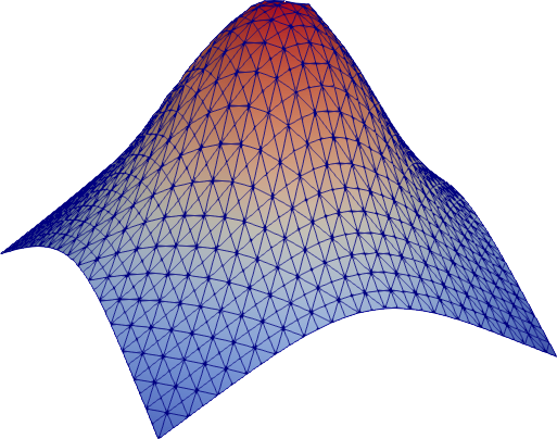
This example approximates a function from _R2_ to _R_ (without noise in the
samples). Note that the absence of noise the data allows us to pick a rather small
`lmbda` such that all sample points are approximated well.
### Comparison with other approaches
#### Polynomial fitting/regression

The classical approach to data fitting is [polynomial
regression](https://en.wikipedia.org/wiki/Polynomial_regression). Polynomials are
chosen because they are very simple, can be evaluated quickly, and [can be made to fit
any function very closely](https://en.wikipedia.org/wiki/Stone–Weierstrass_theorem).
There are, however, some fundamental problems:
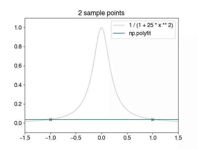
- Your data might not actually fit a polynomial of low degree.
- [Runge's phenomenon](//en.wikipedia.org/wiki/Runge%27s_phenomenon).
This above plot highlights the problem with oscillations.
#### Fourier smoothing

One approach to data fitting with smoothing is to create a function with all data
points, and simply cut off the high frequencies after Fourier transformation.
This approach is fast, but only works for evenly spaced samples.
> [For equidistant curve fitting there is nothing else that could compete with the
> Fourier series.](https://youtu.be/avSHHi9QCjA?t=1543)
> -- Cornelius Lanczos
```python
import matplotlib.pyplot as plt
import numpy as np
rng = np.random.default_rng(0)
# original function
x0 = np.linspace(-1.0, 1.0, 1000)
y0 = 1 / (1 + 25 * x0 ** 2)
plt.plot(x0, y0, color="k", alpha=0.2)
# create sample points
n = 51
x1 = np.linspace(-1.0, 1.0, n) # only works if samples are evenly spaced
y1 = 1 / (1 + 25 * x1 ** 2) + 1.0e-1 * (2 * rng.random(x1.shape[0]) - 1)
plt.plot(x1, y1, "xk")
# Cut off the high frequencies in the transformed space and transform back
X = np.fft.rfft(y1)
X[5:] = 0.0
y2 = np.fft.irfft(X, n)
#
plt.plot(x1, y2, "-", label="5 lowest frequencies")
plt.grid()
plt.show()
```