https://github.com/sixleopard/stable-diffusion

Custom Stable Diffusion Model for ADNI dataset. Generates new Brain MRI's either with or without Alzheimer's Disease depending on input. Could be used as supplimentry data for training an early Alzheimer's Disease detection model
https://github.com/sixleopard/stable-diffusion

adni ai deep-learning meachine-learning nural-network stable-diffusion unet vae variational-autoencoder

Last synced: 2 months ago
JSON representation

Custom Stable Diffusion Model for ADNI dataset. Generates new Brain MRI's either with or without Alzheimer's Disease depending on input. Could be used as supplimentry data for training an early Alzheimer's Disease detection model

• Host: GitHub
• URL: https://github.com/sixleopard/stable-diffusion
• Owner: SixLeopard
• Created: 2025-02-05T10:04:36.000Z (4 months ago)
• Default Branch: main
• Last Pushed: 2025-02-05T10:06:27.000Z (4 months ago)
• Last Synced: 2025-03-31T02:17:37.382Z (2 months ago)
• Topics: adni, ai, deep-learning, meachine-learning, nural-network, stable-diffusion, unet, vae, variational-autoencoder
• Language: Python
• Homepage:
• Size: 4.19 MB
• Stars: 0
• Watchers: 1
• Forks: 0
• Open Issues: 0
• Metadata Files:
  • Readme: README.md

Awesome Lists containing this project

README

        
# Stable Diffusion on ADNI Dataset

## Author

**Jamie Westerhout**

## Description

This is an attempt at an implementation of latent diffusion model based on the stable diffusion architecture to generate new MRI brain scans. The model was trained on the ADNI dataset that contains a total 30520 brain MRI scans in which there are two types of scans AD (Alzheimer’s Disease) labeled as 0 in the results and NC (Normal Control) labeled as 1 in the results. The model is used to generate new MRIs where you can chose if you want a AD type image or an NC type image generated.

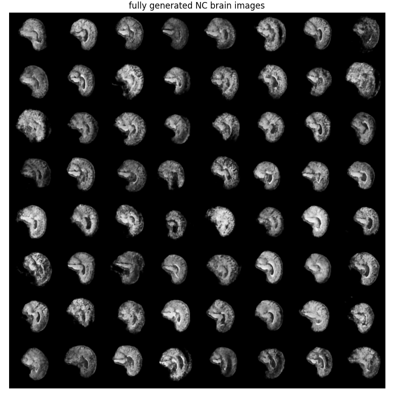
### Sample Fully Generated Output



# Contents

- [File Structure](#File-Structure)

- [Background](#Background)

- [Implementation](#Implementing-Stable-Diffusion)

- [Usage](#Usage)

- [Results](#Results)

- [References](#References)

# File Structure

```

47451933_Stable_Diffusion

├── Results (train results + generation outputs + diagrams)

│   ├── BrainSeq1.png

│   ├── Brains1.png

│   ├── COMP3710SD_diagram.png

│   ├── COMP3710SD_diagram_infrence.png

│   ├── Diffusion_loss.png

│   ├── Diffusion_loss_2.png

│   ├── Diffusion_loss_21.png

│   ├── Diffusion_loss_22.png

│   ├── Diffusion_loss_23.png

│   ├── Diffusion_loss_24.png

│   ├── UMapPlot.png

│   ├── VAE_loss.png

│   ├── VAE_loss_2.png

│   ├── VAE_loss_21.png

│   └── VAE_loss_22.png

│   └── AD_Genrated_Brains.png

│   └── NC_Genrated_Brains.png

│   └── test_brains.png

├── .gitignore

├── README.md

├── dataset.py (for loading in the ADNI dataset)

├── modules.py (contains all the networks)

├── predict.py (use to generate new images)

├── project_setup.py (use to setup folder strucutre and check dataset is avaliable)

├── requirements.txt (what python librariesa re required)

├── train.py (train the model)

└── utils.py (contains extra functions used by most the files)

```

# Background

## Stable Diffusion

Stable diffusion is a generative model and more specifically is a kind of diffusion model call latent diffusion (except for v3 which diverged from latent diffusion). it was developed by Stability AI with help from Runway and CompVis.

# Diffusion Models

Diffusion models are a type of model where images are generated from noise by iteratively removed the noise to construct new images. to train them they are train on the different levels of noise tagged with a time step, these images are then passed to a u-net along with its timestep to try and predict the noise in the images at that timestep. to generate new images a completely noisy image is passed and it goes through every timestep predicting and removing the noise each time. this results in an image completely generated from noise since the u-net is predicting noise that when removed will look like the images its trained on.

Diffusion Models are an alternative to the GAN and standalone VAE approach to generating images. It produces a better variety of images than GANs and better quality images then a VAE but at the cost of slower generation performance 

## Latent Diffusion Models

latent diffusion was developed by researchers at Ludwig Maximilian University and is improvement upon the the diffusion model by since using larger images was extremely slow with diffusion. Latent diffusion can drastically improve the speed by doing the diffusion process in the latent space created by VAE this way its not doing the process on the full image can do it on a down sampled version, thus requiring significantly less resources and time.

# Implementing Stable Diffusion

Stable diffusion V1 is the first stable diffusion model released and has an 8 factor down sampling VAE (Variational Autoencoder), a 860M U-Net and uses OpenAi's CLIP Bit0L/14 text encoder for conditioning on text prompts. 

Exactly replicating one of the stable diffusion model would require significantly more powerful hardware then what is available to train and be significantly overcomplicated due to fact that this model is only required to handle MRI brain scans with 2 labels and for example doesn't need the complexity of the clip encoding since it doesn't need to be able to handle full text descriptions or image inputs etc. 

Since all the original versions of stable diffusion are types of latent diffusion model this is an implementation of stable diffusion's latent diffusion architecture for the ADNI dataset.

## Latent Diffusion Architecture used by Stable Diffusion



this is the latent diffusion architecture used for the original stable diffusion versions.

### Key Components

- Encoder and Decoder to takes images from pixel space to latent space

- Forward diffusion process -> add increasing levels of noise over a set number of timesteps

- De-Noising U-Net to predict the noise of the current timestep

- Cross attention to condition on input

- Denoising step to remove the noise predicted by the u-net

## Model Architecture Implemented



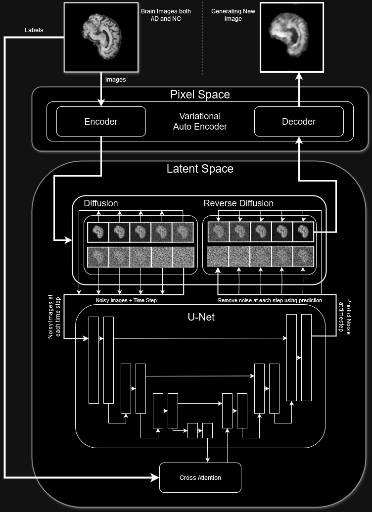
can see the implemented model architecture has all the same key components as the stable diffusion models

### Key Components

- VAE Encoder and Decoder to takes images from pixel space to latent space

- Forward diffusion process -> add increasing levels of noise over a set number of timesteps (using noise schedular + sinusoidal time step embeddings)

- De-Noising U-Net to predict the noise of the current timestep

- Cross attention to condition on whether the brain is AD or NC

- Denoising step to remove the noise predicted by the u-net

## Setup

### Train, Test, Validation Split

the ADNI dataset comes with a train test split already but having an additional validation set is useful to see generalization performance during training to see if the model is overfitting. Since the images are broken up between a patient and then all the slices of there brain to split the data into an additional set is not as easy as just taking a 10% extra split off since this would result in images data leakage. so to get an additional validation set the test set was split using the following algorithm (in sudo code):

```python

num_patients_for_val_set = num_images_in_train_set // 100

patients_seen = set()

for i in test_set:

    patient = i.split("_")[0]

    if len(patients_seen) <= num_patients_for_val_set:

        patients_seen.add(patient)

    if patient in patients_seen:

        move_from_test_to_val(i)

```

the original train set was used as the train set then what was left of the test set about 11k images was used for testing and for validation the new validation set created was used

### Data Transformations

the following transformation were applied to the images before loading

```python

transforms = tvtransforms.Compose([

            tvtransforms.Grayscale(), #grascale images 

            tvtransforms.Resize(self.image_size), #the next two lines decrease the resolution to 200x200

            tvtransforms.CenterCrop(self.image_size),

            tvtransforms.ToTensor(), #turn the datat into a tensor if its not already

            tvtransforms.Normalize(0.5,0.5)]) #normilze the data

```

- the grey scale takes the images from 3 channels to 1 channel reducing the size of each image without loss of information because there grey scale anyway

- resize to 200x200 since there originally 256x240 so cropped to 200x200 to make them square to simplify things and slightly reduce the size of each image

- normalize the images otherwise this could cause poor performance

### Batchs

The data was batched into batches of size 128 useing dataloaders, this was chosen as its large enough that it should include most of the different layers of slices in each batch and was the largest that would fit on an 8Gb Vram GPU during training.

# Usage

before running either the training or predicting run the setup.py first to make sure all the correct folders are created for the models to save to when completed and it also check to make sure the dataset is present and in the right location and format

## Training

The the VAE for encoding and decoding is train separately from the u-net since it isn't reasonable for them both to be trained at the same since the u-net relies on latent space produced from the VAE to train and if this is changing at the same time it won't learn properly. First the VAE is trained to encode images into latent space in this case since its a vae it produces a distribution over the latent space, it then reconstruct from a sample of the distribution.

### Overall Choices

- AdamW was used as the optimizer of both the VAE and U-net since its an improvement on the already good Adam but addressing its main problem of not generalizing well by decoupling the weight decay from the gradient update.

- CosineAnnealingLR was used as the learning rate schedualar for both the VAE and U-Net again since its method of increasing and decreasing the lr periodically to make it explore then learn makes it more likely to reach the global minium during sgd.

### VAE Training

Trained to be able to encode and decode the image trying to get as similar output to the image it put in.

#### Encoding

each image is encoded using the vea which then produces a mu and logvar for the latent space, to actually get an encoded image, a sample is taken from this latent space which also output as h

(sudo codified for isolated interpretability)

```python

# get mean and variance for sampling

# and to be used to calculate Kullback-Leibler divergence loss.

h = self.encoder(x)

mu = self.fc_mu(h)

logvar = self.fc_logvar(h)

# get sample

z = self.sample_latent(mu, logvar)

h = self.decode(z)

return h, mu, logvar

```

#### Decoding

after each image goes through the encoder the sample h then gets put through the decoder, to reconstruct the image

(sudo codified for isolated interpretability)

```python

x_recon = self.decoder(z)

return x_recon

```

#### Loss

the loss for a vae is combination of the construction loss and Kullback-Leibler divergence loss to not only ensure that its reconstructing the images well by the KL loss works like regularization ensuring that's its generalizing well by measuring the distribution its producing

(sudo codified for isolated interpretability)

```python

#sudo code

reconstrcution_loss = MSE(reconstructed_images, images, reduction='sum')

Kullback-Leibler_divergence_loss = -0.5 * torch.sum(1 + logvar - mu.pow(2) - logvar.exp())

loss = 0.5*recon_loss + Leibler_divergence_loss

```



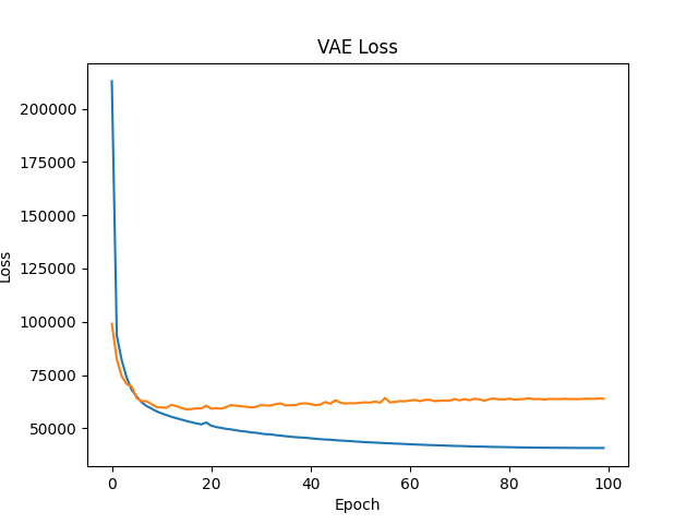
can see that the validation loss increases after about 20 epochs so probably some overfitting but it doesn't really increase much.

### U-Net Training

The u-net is trained to take an encoded image that has had a noise added to it in the latent then predict what the noise was so then it can be removed so it can be decoded to get back the original image

#### Encoding

Before being able to pass an image into the u-net for training it has be encoded into the latent space as the U-Net

(sudo codified for isolated interpretability)

```python

z, _, _ = vae_encoder(images)

```

#### Forward Diffusion (adding noise)

at each step of train a random timestep is chosen then the noise scheduler is used to determine how much noise should be added for that timestep. the noises is then added:

(sudo codified for isolated interpretability)

```python

def add_noise(x, t, nosie_schedular):

    #create random noise sampled from normal distibution

    noise = torch.randn_like(x).to(device)

    #get cumulative product of the amounts up to time t

    alpha_t = nosie_schedular.get_alphas_cumprod()[t].to(x.device)

    #squre root of it

    sqrt_alpha_t = torch.sqrt(alpha_t)

    #inverse of it

    sqrt_beta_t = torch.sqrt(1 - alpha_t)

    #add it in a way that the noise being added doesn't

    #keep just brighting the image

    return sqrt_alpha_t * x + sqrt_beta_t * noise, noise

noisy_latent, noise = add_noise(z, t, noise_scheduler)

```

#### U-Net noise prediction

now that there is noise added to the latent image then use the u-net to predict the noise that was added

(sudo codified for isolated interpretability)

```python

predicted_noise, _ = unet(noisy_latent, labels, t)

```

this noise is then compared to the noise that was added and how far off it was determines the loss

#### Loss

loss function used is MSE to compare the predict noise to the real noise added

(sudo codified for isolated interpretability)

```python

loss = MSE(predicted_noise, noise)

```

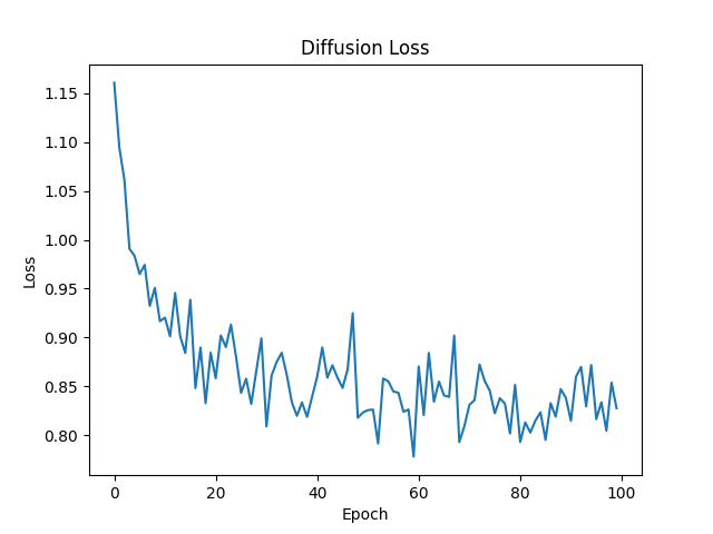
diffusion loss over 100 epochs



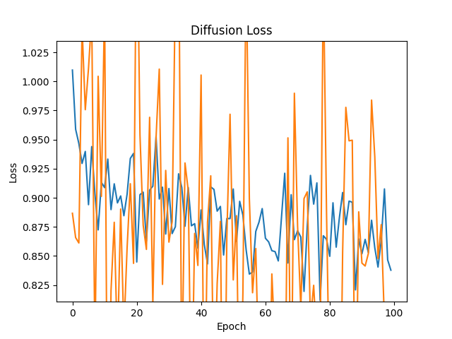
can see that the validation loss is super noisy by still follows a general trend down, likely because the validation is a lot smaller then the training set.



What it looks like without validation set covering it

## Inference

inference works a bit different to what is done in training since when training the images are being input but when doing inference, want to produce and entire new image from nothin so input is just random noise in the shape of latent space 



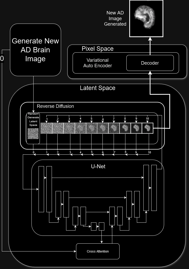
This random noise then goes through the reverse diffusion process and decoded to generate a new image entirely from noise

#### Reverse Diffusion

the reverse diffusion process takes the fully noisy image and predict the noise add at each time step so first it gets the noise predicted for it at timestep 10 then gets the noise removed, it then gets predicted for timestep 9 then removed ......

this is what the process looks like in code (sudo codified for isolated interpretability)

```python

#genete a tensor with the given label for the number of images to generate

label = torch.tensor([label] * num_samples).to(device)

with torch.no_grad():

	#generate ranom latent

	x = torch.randn(num_samples, latent_dim).to(device)

	#turn latent form the 2 dim to 3 dim version

	x = vae_encoder.decode(x)

	for t in reversed(range(num_timesteps)):

		#predict noise for the timestep

		predicted_noise, _ = Unet(x, label, t)

		#remove noise for rhe timestep

		x = denoise(x, predicted_noise, t, nosie_schedular)

```

#### Decoding

after going through the reverse diffusion what is left is theoretically a latent vector that when decoded should produce a good brain image conditioned on the label 

(sudo codified for isolated interpretability)

```python

output_image = vae_decoder(denoised_latent)

```

#### Results





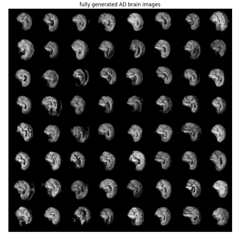
can't easily tell a difference between the AD and NC output but couldn't either with the original images. overall the images look like brains and are of reasonable quality. It is obviously generating new ones with some having some weird extra features and patterns within that aren't quite completely realistic. 

# Reproducing Results

to reproduce the results in this readme,

1. Download ADNI data set and put in a folder called data in the directory (follow setup.py instructions)

2. Run train.py to train both the VAE and U-Net

3. Run predict.py to generate new images

results wont look exactly the same due to it being a generative model and variation in training runs but should get something very similar.

could also train for more epochs then  the default which is set at 100 and could possibly get higher quality images 

## Umap Embedding Plot

to see to make sure that the label conditioning is happen properly, At the U-Net bottleneck the there is a clear division in the data that's labeled as AD and the ones labeled NC. To ensure that its actually conditioning the outputs. Due to it being in the latent space it cant easily be displayed as its 128 dimensional space then passed through half a U-Net so to actually visualize it going to be using Umap.



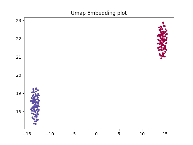
can see theirs a clear distinction between the two as intended.

## Dependencies

all the packages installed when doing all the training and testing of the models is included in the requirements.txt file install this file with pip before use will ensure everything will work as expected.

# References

- ADNI | Alzheimer’s Disease Neuroimaging Initiative (no date) ADNI. Available at: https://adni.loni.usc.edu/. (ADNI dataset)

- Rombach, R. et al. (2022) ‘High-Resolution Image Synthesis with Latent Diffusion Models’, arXiv:2112.10752 [cs] [Preprint]. Available at: https://arxiv.org/abs/2112.10752. (stable diffusion paper)

- Stable Diffusion (2022) GitHub. Available at: https://github.com/CompVis/stable-diffusion. (stable diffusion repo)

- McInnes, L., Healy, J. and Melville, J. (2018) UMAP: Uniform Manifold Approximation and Projection for Dimension Reduction, arXiv.org. Available at: https://arxiv.org/abs/1802.03426. (umap paper)