https://github.com/stephane-caron/qpmpc
Model predictive control in Python based on quadratic programming
https://github.com/stephane-caron/qpmpc
linear-time-invariant linear-time-variant model-predictive-control optimal-control python trajectory-optimization
Last synced: 10 months ago
JSON representation
Model predictive control in Python based on quadratic programming
- Host: GitHub
- URL: https://github.com/stephane-caron/qpmpc
- Owner: stephane-caron
- License: apache-2.0
- Created: 2022-03-30T14:06:55.000Z (about 4 years ago)
- Default Branch: main
- Last Pushed: 2025-03-11T11:13:30.000Z (over 1 year ago)
- Last Synced: 2025-03-15T03:38:04.546Z (over 1 year ago)
- Topics: linear-time-invariant, linear-time-variant, model-predictive-control, optimal-control, python, trajectory-optimization
- Language: Python
- Homepage:
- Size: 337 KB
- Stars: 37
- Watchers: 2
- Forks: 1
- Open Issues: 0
-
Metadata Files:
- Readme: README.md
- Changelog: CHANGELOG.md
- Contributing: CONTRIBUTING.md
- License: LICENSE
Awesome Lists containing this project
README
# qpmpc
[](https://github.com/stephane-caron/qpmpc/actions)
[](https://scaron.info/doc/qpmpc/)
[](https://coveralls.io/github/stephane-caron/qpmpc?branch=main)
[](https://anaconda.org/conda-forge/qpmpc)
[](https://pypi.org/project/qpmpc/0.6.0/)
Model predictive control (MPC) in Python for optimal-control problems that are quadratic programs (QP). This includes linear time-invariant (LTI) and time-variant (LTV) systems with linear constraints. The corresponding QP has the form:
> 
This module is designed for prototyping. If you need performance, check out the [alternatives](#alternatives) below.
## Installation
```sh
pip install qpmpc
```
## Usage
This module defines a one-stop shop function:
```python
solve_mpc(problem: MPCProblem, solver: str) -> Plan
```
The [``MPCProblem``](https://scaron.info/doc/qpmpc/usage.html#qpmpc.mpc_problem.MPCProblem) defines the model predictive control problem (LTV system, LTV constraints, initial state and cost function to optimize) while the returned [``Plan``](https://scaron.info/doc/qpmpc/usage.html#qpmpc.plan.Plan) holds the state and input trajectories that result from optimizing the problem (if a solution exists). The ``solver`` string is used to select the backend [quadratic programming solver](https://github.com/stephane-caron/qpsolvers#solvers).
## Example
Let us define a triple integrator:
```python
import numpy as np
horizon_duration = 1.0 # [s]
N = 16 # number of discretization steps
T = horizon_duration / N
A = np.array([[1.0, T, T ** 2 / 2.0], [0.0, 1.0, T], [0.0, 0.0, 1.0]])
B = np.array([T ** 3 / 6.0, T ** 2 / 2.0, T]).reshape((3, 1))
```
Suppose for the sake of example that acceleration is the main constraint acting on our system. We thus define an acceleration constraint ``|acceleration| <= max_accel``:
```python
max_accel = 3.0 # [m] / [s] / [s]
accel_from_state = np.array([0.0, 0.0, 1.0])
C = np.vstack([+accel_from_state, -accel_from_state])
e = np.array([+max_accel, +max_accel])
```
This leads us to the following linear MPC problem:
```python
from qpmpc import MPCProblem
x_init = np.array([0.0, 0.0, 0.0])
x_goal = np.array([1.0, 0.0, 0.0])
problem = MPCProblem(
transition_state_matrix=A,
transition_input_matrix=B,
ineq_state_matrix=C,
ineq_input_matrix=None,
ineq_vector=e,
initial_state=x_init,
goal_state=x_goal,
nb_timesteps=N,
terminal_cost_weight=1.0,
stage_state_cost_weight=None,
stage_input_cost_weight=1e-6,
)
```
We can solve it with:
```python
from qpmpc import solve_mpc
solution = solve_mpc(problem, solver="proxqp")
```
The solution holds complete state and input trajectories as stacked vectors. For instance, we can plot positions, velocities and accelerations as follows:
```python
import pylab
t = np.linspace(0.0, horizon_duration, N + 1)
X = solution.states
positions, velocities, accelerations = X[:, 0], X[:, 1], X[:, 2]
pylab.ion()
pylab.plot(t, positions)
pylab.plot(t, velocities)
pylab.plot(t, accelerations)
pylab.grid(True)
pylab.legend(("position", "velocity", "acceleration"))
```
This example produces the following trajectory:
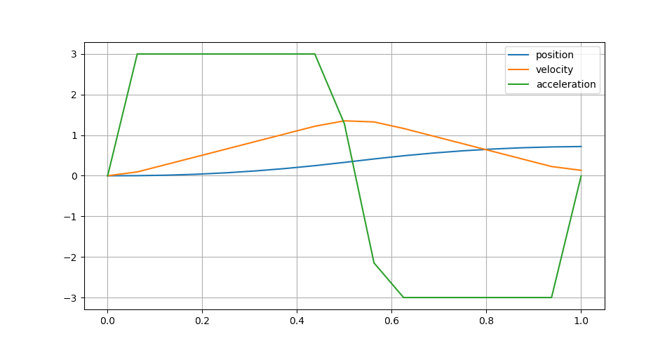
The behavior is a weighted compromise between reaching the goal state (weight ``1.0``) and keeping reasonable finite jerk inputs (weight ``1e-6``). The latter mitigate bang-bang accelerations but prevent fully reaching the goal within the horizon. See the [examples](examples/) folder for more examples.
## Areas of improvement
This module is incomplete with regards to the following points:
- Cost functions: can be extended to general linear stage cost functions
- Documentation: there are some undocumented functions
- Test coverage: only one end-to-end test
Check out the [contribution guidelines](CONTRIBUTING.md) if you are interested in lending a hand.
## Alternatives
You can also check out the following open-source libraries:
### Linear model predictive control
| Name | Systems | Languages | License |
|------------------------------------------------------------|-----------------------|-------------|--------------|
| [Copra (LTV fork)](https://github.com/ANYbotics/copra) | Linear time-variant | C++, Python | BSD-2-Clause |
| [Copra (original)](https://github.com/jrl-umi3218/copra) | Linear time-invariant | C++, Python | BSD-2-Clause |
| [mpc-interface](https://github.com/Gepetto/mpc-interface) | Linear time-variant | C++, Python | BSD-2-Clause |
| [pyMPC](https://github.com/forgi86/pyMPC) | Linear time-variant | Python | MIT |
### Nonlinear model predictive control
| Name | Systems | Languages | License |
|------------------------------------------------------------|-----------------------|---------------------|--------------|
| [acados](https://github.com/acados/acados) | Nonlinear | C++, Matlab, Python | BSD-2-Clause |
| [Aligator](https://github.com/Simple-Robotics/aligator/) | Nonlinear | C++, Python | BSD-2-Clause |
| [Crocoddyl](https://github.com/loco-3d/crocoddyl) | Nonlinear | C++, Python | BSD-3-Clause |