https://github.com/vdemichev/DiaNN

DIA-NN - a universal automated software suite for DIA proteomics data analysis.
https://github.com/vdemichev/DiaNN

Last synced: about 1 year ago
JSON representation

DIA-NN - a universal automated software suite for DIA proteomics data analysis.

Host: GitHub
URL: https://github.com/vdemichev/DiaNN
Owner: vdemichev
License: other
Created: 2018-03-14T22:46:20.000Z (about 8 years ago)
Default Branch: master
Last Pushed: 2025-03-25T11:52:44.000Z (about 1 year ago)
Last Synced: 2025-03-25T12:21:46.892Z (about 1 year ago)
Language: C++
Homepage:
Size: 260 MB
Stars: 331
Watchers: 24
Forks: 61
Open Issues: 529
Metadata Files:
- Readme: README.md
- License: LICENSE.md

Awesome Lists containing this project

awesome-proteomics - DIA-NN - C/C++ - free and open source search tool for DIA data that uses neural networks, works using either a library or a FASTA database. - [paper](https://www.nature.com/articles/s41592-019-0638-x) (3. Raw data search software/algorithms / Table of Contents)

README

DIA-NN

DIA-NN is an automated software suite for data-independent acquisition (DIA) proteomics data processing.

DIA-NN is built on the following principles:
- **Reliability** achieved via stringent statistical control
- **Robustness** achieved via flexible modelling of the data and automatic parameter selection
- **Reproducibility** promoted by thorough recording of all analysis steps
- **Ease of use**: high degree of automation, an analysis can be set up in several mouse clicks, no bioinformatics expertise required
- **Powerful tuning options** to enable unconventional experiments
- **Scalability and speed**: up to 1000 mass spec runs processed per hour

**Download DIA-NN 2.1.0** for academic research: https://github.com/vdemichev/DiaNN/releases/tag/2.0.
**DIA-NN 2.1.0 Enterprise** for industry use: contact Aptila Biotech [aptila.bio](https://www.aptila.bio) to purchase or obtain a trial license.

### Table of Contents
**[Installation](#installation)**

**[Getting started with DIA-NN](#getting-started-with-dia-nn)**

**[Changing default settings](#changing-default-settings)**

**[Raw data formats](#raw-data-formats)**

**[Spectral library formats](#spectral-library-formats)**

**[Sequence databases](#sequence-databases)**

**[Output](#output)**

**[Command interface](#command-interface)**

**[Visualisation](#visualisation)**

**[Automated pipelines](#automated-pipelines)**

**[PTMs and peptidoforms](#ptms-and-peptidoforms)**

**[Fine tuning prediction models](#fine-tuning-prediction-models)**

**[Multiplexing using plexDIA](#multiplexing-using-plexdia)**

**[Editing spectral libraries](#editing-spectral-libraries)**

**[Custom decoys](#custom-decoys)**

**[Integration with other tools](#integration-with-other-tools)**

**[Quantification](#quantification)**

**[Speed optimisation](#speed-optimisation)**

**[Incremental processing](#incremental-processing)**

**[Basics of DIA data analysis](#basics-of-dia-data-analysis)**

**[GUI settings reference](#gui-settings-reference)**

**[Command-line reference](#command-line-reference)**

**[Main output reference](#main-output-reference)**

**[Frequently asked questions](#frequently-asked-questions)**

**[Support](#support)**

**[Key publications](#key-publications)**

### Installation

On **Windows**, download and run the .msi file. It is recommended to install DIA-NN into the default folder suggested by the installer. If your system may not have the common packages from Microsoft installed, download and run [https://aka.ms/vs/17/release/vc_redist.x64.exe](https://aka.ms/vs/17/release/vc_redist.x64.exe), [https://go.microsoft.com/fwlink/?linkid=863265](https://go.microsoft.com/fwlink/?linkid=863265) as well as [https://dotnet.microsoft.com/en-us/download/dotnet/thank-you/sdk-8.0.407-windows-x64-installer](https://dotnet.microsoft.com/en-us/download/dotnet/thank-you/sdk-8.0.407-windows-x64-installer) and reboot your PC.

On **Linux** (command-line use only), download and unpack the Linux .zip file. The Linux version of DIA-NN is generated on Linux Mint 21.2, and the target system must have the standard libraries that are at least as recent. There is no such requirement, however, if you make a Docker or Apptainer/Singularity container image. To generate either container, we recommend starting with the latest debian docker image, the script make_docker.sh that does this is included. You can also check the excellent [guide](https://github.com/vdemichev/DiaNN/issues/1202#issuecomment-2417108281) by Roger Olivella. See [Command interface](#command-interface) for Linux-specific usage guidance.

It is also possible to run DIA-NN on Linux using **Wine** 6.8 or later.

### Getting Started with DIA-NN

If you are new to DIA proteomics, please take a look at the [Basics of DIA data analysis](#basics-of-dia-data-analysis).

DIA-NN analysis consists of two steps. First, use DIA-NN to generate a **predicted spectral library** from the sequence database, this library can then be reused for all experiments involving the **respective organism**. This first step is not necessary if you have a suitable **empirical spectral library** (e.g. generated by DIA-NN based on analysis of some DIA experiment). Second, have DIA-NN analyse the raw data with the selected spectral library. Each of the steps is set up in just several mouse clicks.

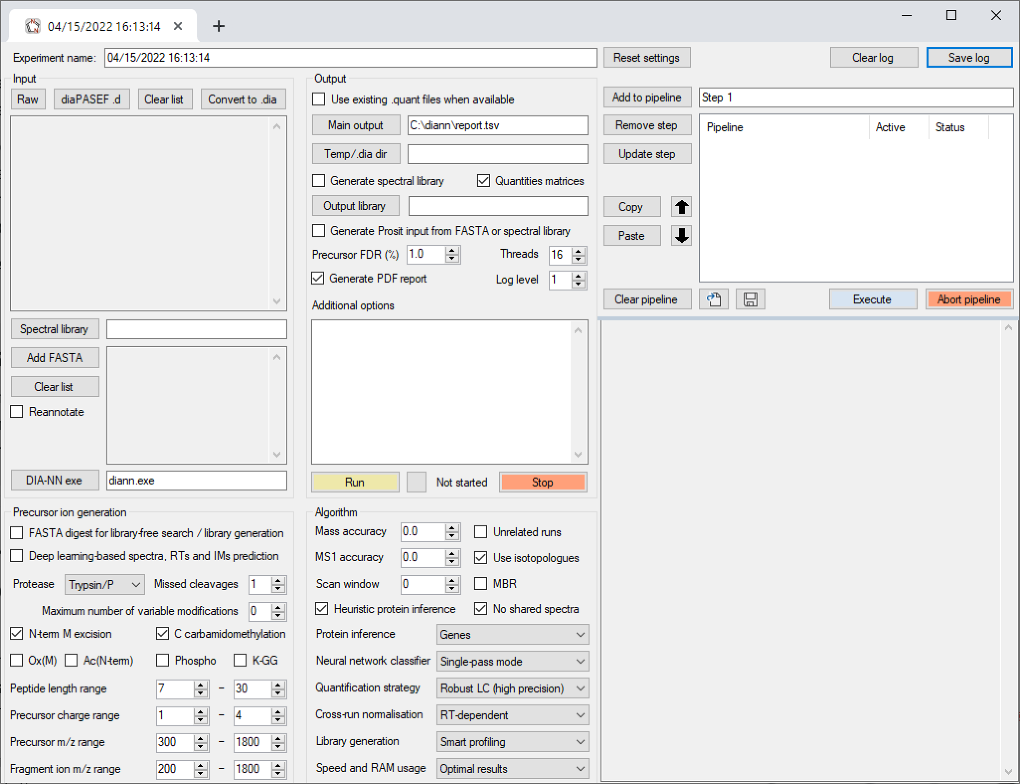
**Predicted library generation**:
1. Click **Add FASTA**, add one or more sequence databases in UniProt format.
2. Check **FASTA digest** checkbox. The **Deep learning** checkbox below gets checked automatically.
3. (Optional) You can edit the **Output library** field. This is in fact a name 'template'. In workflows that generate empirical DIA-based libs, these are saved in the Apache .parquet format as specified by **Output library**. However, in this case DIA-NN will be generating a predicted library as specified by **Predicted library** below - it is the same name template, but the file has a different extension - .predicted.speclib, which is DIA-NN's own compact binary format for spectral libraries.
4. Click **Run**. DIA-NN's log will be displayed in the log field (large field occupying the bottom-right part of the GUI window). Library generation takes less than 2 minutes per million precursors on a modern 16-core desktop CPU.

**Analysing with (any) spectral library**:
1. Click **Spectral library** and specify the library to use. Can be the .predicted.speclib as generated above, a .parquet lib generated by some previous DIA-NN analysis or some third-party predicted or empirical library in a compatible format (more about these below).
2. Click **Add FASTA**, add one or more sequence databases in UniProt format, corresponding to the spectral library (i.e. if the library contains human proteins, any human database is fine here). If the library does not contain correct protein information (e.g. some third-party library), check **Reannotate**, this will update the protein information for each of the precursors in the library.
3. Click **Raw** and select the raw data files. In case of Bruker timsTOF data, click instead **.d (DIA)** and specify the timsTOF acquisitions (which are folders with names ending with .d).
4. (Optional) Adjust **Main output**. This is the name of the main output report generated by DIA-NN. It is also used by DIA-NN as the name template for any other report files it is going to generate (more about these below).
5. Click **Run**. Note that DIA-NN will use the raw data to generate an empirical spectral library (file name specified by **Output library**).

If it is your very first time running DIA-NN, it makes sense to first explore how DIA-NN output looks like. For this, run DIA-NN on a dataset that can be analysed just in a couple of minutes. We recommend downloading raw data files (dia-PASEF 10ng.zip archive), empirical spectral library (K562-spin-column-lib.zip) and a FASTA database (human_canonical_uniprotkb_proteome_UP000005640_2023_12_16.fasta) from the [Slice-PASEF benchmarks repository](https://osf.io/t2ymc/?view_only=7462fffb20e648fc83afc75d8c67e9f8). When analysing this dataset, uncheck the **MBR** and **Generate spectral library** checkboxes.

**Output**:
- The DIA-NN main report contains a list of all precursors ('Precursor.Id' column), with respective matched proteins ('Protein.Group' column) and quantities for both precursor and proteins ('Precursor.Normalised' and 'PG.MaxLFQ', respectively), for each run in the experiment. The report is in a .parquet format, it is basically a way to store text tables in a compact compressed format, it can be accessed with either R 'arrow' or Python 'pyarrow' or 'polars' packages.

- In case you would like to immediately take a look at the protein quantities table, using software such as MS Excel, DIA-NN generates simple ready-to-use .pg_matrix.tsv and .unique_genes_matrix.tsv tab-separated tables of quantities.

The above information is sufficient for one to start using DIA-NN, it's indeed this easy! Please also check the [Visualisation](#visualisation) and [Automated pipelines](#automated-pipelines) sections, these describe some very helpful functionality of the DIA-NN GUI, as well as [Changing default settings](#changing-default-settings) below.

### Changing default settings

**LC-MS-specific parameters**. for publication-ready analyses, it is preferable to adjust the mass accuracies and the 'scan window' used by DIA-NN. These parameters provide guidance to DIA-NN, informing it on the expected magnitude of mass deviations (mass accuracies) and the expected number of DIA cycles per the average peptide elution time. By default, these are set to 0, meaning that DIA-NN will optimise them automatically for the first run in the experiment and then reuse the optimised settings for other runs. This optimisation process is 'noisy' in the sense that even replicate injections may not produce identical results. Therefore, the analysis results will depend on which run is first in the list of raw data files provided to DIA-NN. It's preferable to rather fix these three parameters to values know to be optimal for a particular LC-MS setup:

1. If the data were generated on timsTOF, set both **Mass accuracy** (MS/MS mass tolerance) and **MS1 accuracy** (MS1 mass tolerance) to 15.0 (ppm). Note that these settings provide a 'guidance' to DIA-NN, the actual m/z window used to match theoretical m/z values to the (m/z, intensity) pairs in the raw data file will be specific to both the precursor and the raw data in the vicinity of its putative retention time.

2. If the data were generated on Oritrap Astral, set **Mass accuracy** to 10.0 and **MS1 accuracy** to 4.0.

3. If the data were generated on TripleTOF 6600 or ZenoTOF, set **Mass accuracy** to 20.0 and **MS1 accuracy** to 12.0.

4. In other cases (e.g. Q Exactive and Exploris mass spectrometers) or if you would like to optimise everything to squeeze the best possible performance from the data, run DIA-NN on several representative runs (best to use any suitable empirical library, as this is the quickest) with **Unrelated runs** option checked and see what 'Optimised mass accuracy' and 'Recommended MS1 mass accuracy' it reports for those runs in the log.

5. Set **Scan window** to the approximate number of DIA cycles during the elution time of an average peptide. You can also have DIA-NN suggest the optimal one using an analysis with **Unrelated runs** checked.

**How to interpret the rest of the present guide**. The above covers DIA-NN use for 95% of projects. However, DIA-NN also offers powerful tuning options for fancy experiments. If you are just starting with DIA-NN, we recommend to first run it on a couple of simple datasets to get a feeling of how it works and then skim through the rest of this guide to see if any tips here can also be useful for your applications. The whole guide takes about 15 minutes to skim through and about 1-2 hours to study in detail.

In general, we recommended to:
- Only change the default settings if (i) the change is recommended in the present guide, or (ii) you know that the change is necessary for your type of experiment and it's not covered in this guide, or (iii) you have already tested the default settings and you would like to see the effect of alternative settings.

- Examine DIA-NN's log for warnings/errors. The warnings and errors are printed when they occur as well as at the end of the log, i.e. you can immediately see them once the DIA-NN analysis finishes.

- DIA-NN prints some comments on the settings used at the top of the log, examine these the first time you use the settings to see if there are any recommendations.

The rest of this guide references extra options/commands you can pass to DIA-NN, please see [Command interface](#command-interface) for an introduction.

### Raw data formats

Formats supported: Sciex .wiff, Bruker .d, Thermo .raw, .mzML and .dia (format used by DIA-NN to store spectra). Conversion from any supported format to .dia is possible (except for Slice-type acqusitions on timsTOFs). When running on Linux (native builds, not Wine), only .d, .raw, .mzML, and .dia data are supported.

For .wiff support, download and install [ProteoWizard](http://proteowizard.sourceforge.net/download.html) - choose the version (64-bit) that supports "vendor files"). Then copy all files with 'Clearcore' or 'Sciex' in their name (these will be .dll files) from the ProteoWizard folder to the DIA-NN installation folder (the one which contains diann.exe, DIA-NN.exe and a bunch of other files).

.mzML files should be centroided and contain data as spectra (e.g. SWATH/DIA) and not chromatograms.

Technology support

- DIA and SWATH are supported
- Acquisition schemes with overlapping windows are supported
- Gas-phase fractionation is supported
- Scanning SWATH and ZT Scan DIA are supported
- dia-PASEF/py-diAID are supported
- Slice-PASEF is supported
- midia-PASEF is supported
- Synchro-PASEF/VistaScan is supported, however accuracy of quantitation needs to be validated with benchmarks
- Orbitrap Astral is supported
- FAIMS with constant CV is supported
- multiplexing with non-isobaric tags and SILAC is supported
- MSX-DIA is not supported

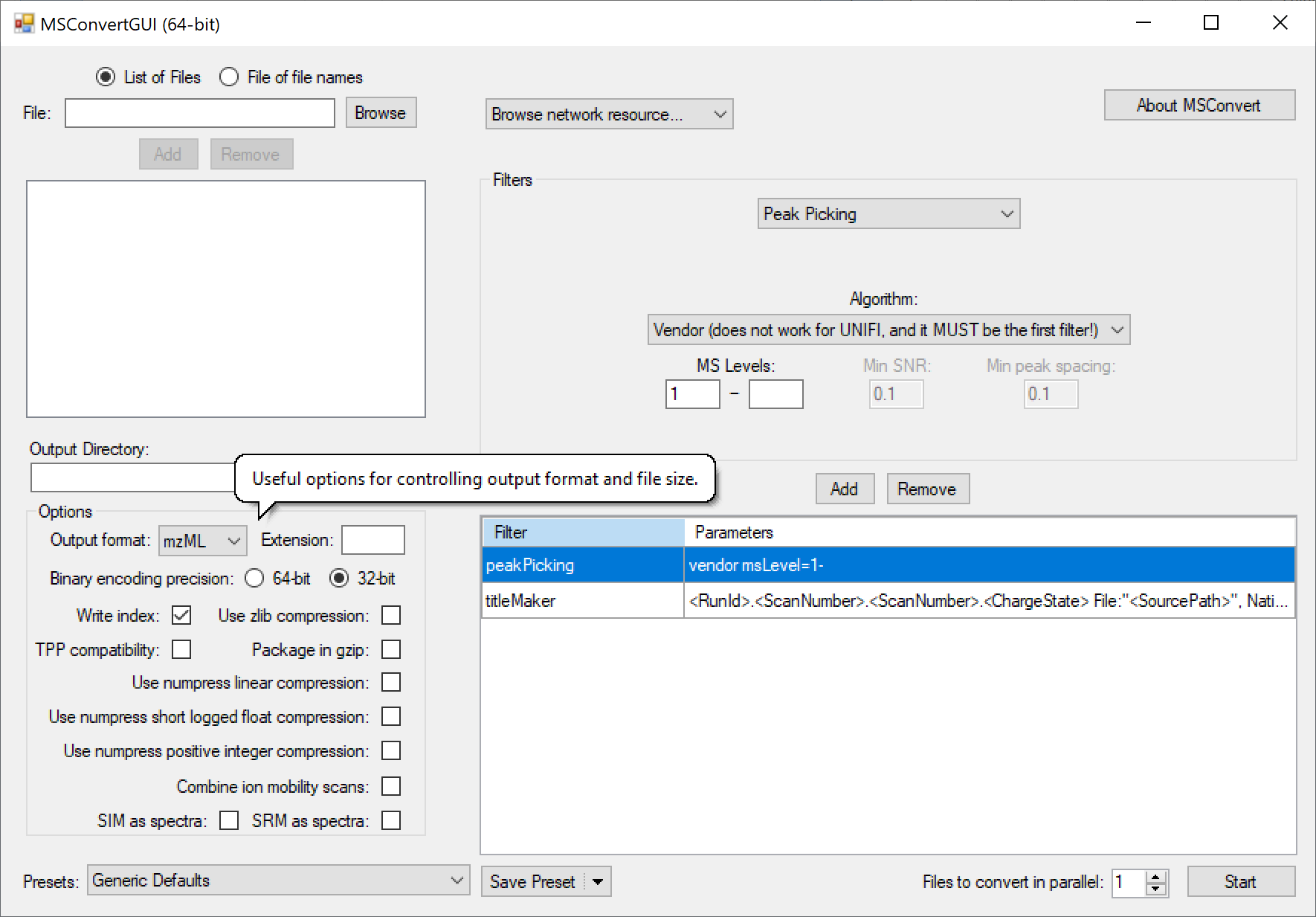
Conversion

Many mass spec formats, including those few that are not supported by DIA-NN directly, can be converted to .mzML using the MSConvertGUI application from [ProteoWizard](http://proteowizard.sourceforge.net/download.html). This works for all supported formats except Bruker .d and SCIEX Scanning SWATH or ZT Scan DIA - these need to be accessed by DIA-NN directly. The following MSConvert settings must be used for conversion:

### Spectral library formats

DIA-NN supports comma-separated (.csv), tab-separated (.tsv, .xls or .txt) or .parquet tables as spectral libraries, as well as .speclib (compact format used by DIA-NN).

In detail

Libraries in the PeakView format as well as libraries produced by FragPipe, TargetedFileConverter (part of OpenMS) are supported “as is”, however compatibility needs to be verified in each particular case (third party software version, its settings and the type of raw data).

DIA-NN can convert any library it supports into its own .parquet format. For this, click **Spectral library** (**Input** pane), select the library you want to convert, select the **Output library** file name (**Output** pane), click **Run**. If you use some exotic library format, it's a good idea to convert it to DIA-NN's .parquet and then examine the resulting library (using R 'arrow' or Python 'pyarrow' package) to see if the contents make sense.

All .tsv/.xls/.txt/.csv/.parquet libraries are just simple tables with human-readable data, and can be explored/edited, if necessary, using Excel or (ideally) R/Python. When editing and then saving DIA-NN's .parquet libraries, make sure to verify that the column types in the schema are unchanged: all floating point columns must be of the FLOAT parquet type and all integer columns must be of the INT64 parquet type.

### Sequence databases

DIA-NN accepts sequence databases in uncompressed FASTA format. The UniProt format is fully supported. For sequence databases in other formats, DIA-NN will most likely correctly extract the information on protein sequence IDs, however it may not correctly read the protein names, gene names and protein descriptions. In such cases, we recommend using any R package meant for handling FASTA databases to reformat the database in UniProt format.

### Output

The **Output** pane allows to specify where the output should be saved as well as the file names for the main output report and (optionally) the output spectral library. DIA-NN uses these file names to derive the names of all of its output files. Below one can find information on different types of DIA-NN output. For most workflows one only needs the main report (for analysis in R or Python - recommended) or the matrices (simplified output for MS Excel). When the generation of output matrices is enabled, DIA-NN also produces a .manifest.txt file with a brief description of the output files generated.

Main report

A text table in .parquet format containing precursor and protein IDs, as well as plenty of associated information. Please use either R "arrow" or Python "pyarrow"/"polars" packages to process. In addition to using R or Python, you can also view .parquet files with the [TAD Viewer](https://www.tadviewer.com/). Similarly to R/Python, this app can be used to export .parquet to .csv.

Most column names are self-explanatory, and the full reference as well as guidance on how to filter the main report can be found in [Main output reference](#main-output-reference). The following keywords are used when naming columns:
- **PG** means protein group
- **GG** means gene group
- **Quantity** means non-normalised quantity
- **Normalised** means normalised quantity
- **TopN** means normalised protein quantity calculated using the TopN method when the **Quantification strategy** is set to **Legacy (direct)**, using these is usually not recommended
- **MaxLFQ** means normalised protein quantity calculated using QuantUMS (**Quantification strategy** set to one of **QuantUMS** modes) or the MaxLFQ (**Quantification strategy** set to **Legacy (direct)**) algorithm, using quantities in this column is recommended for most applications
- **Global** refers to a global q-value, that is calculated for the entire experiment
- **Lib** refers to the respective value saved in the spectral library, e.g. Lib.Q.Value means q-value for the respective library precursor; when using **MBR**, **Lib** q-values will correspond to q-values in the empirical DIA-based lib created in the first pass of **MBR**

Matrices

These contain normalised QuantUMS or MaxLFQ quantities for protein groups ('pg_matrix'), gene groups ('gg_matrix'), unique genes ('unique_genes_matrix'; i.e. genes identified and quantified using only proteotypic, that is gene-specific, peptides) as well as normalised quantities for precursors ('pr_matrix'). They are filtered at 1% FDR, using global q-values for protein groups and both global and run-specific q-values for precursors. Additional 5% run-specific protein-level FDR filter is applied to the protein matrices, use --matrix-spec-q to adjust it. Sometimes DIA-NN will report a zero as the best estimate for a precursor or protein quantity. Such zero quantities are omitted from protein/gene matrices. Special phosphosite quantification matrices (phosphosites_90 and phosphosites_99 .tsv) are generated when phosphorylation (UniMod:21) is declared as a variable modification, see [PTMs and peptidoforms](#ptms-and-peptidoforms).

Protein description

The .protein_description.tsv file is generated along with the Matrices and contains basic protein information known to DIA-NN (sequence IDs, names, gene names, description, sequence). Future versions of DIA-NN will include more information, e.g. protein molecular weight.

Stats report

Contains a number of QC metrics which can be used for data filtering, e.g. to exclude failed runs or as a readout for method optimisation. Note that the number of proteins reported here corresponds to the number of unique proteins (i.e. identified with proteotypic precursors) in a given run at 1% unique protein q-value. This number can be reproduced from the main report generated using precursor FDR threshold of 100% and filtered using Protein.Q.Value <= 0.01 & Proteotypic == 1. What's counted as 'protein' here depends on the 'Protein inference' setting.

PDF reports

Two PDF reports, one containing QC metrics for each acquisition, another with trends observed over the experiment. The PDF reports are generated automatically on Windows, on Linux you can use Python to invoke the diann-stats.py script (located next to the diann-linux binary). Please note that the PDF reports are meant to provide quick quality control for the experiment. If you would like to use them in a publication, please examine the diann-stats.py script for exact definition of what is being plotted by the report.

Flexible reanalysis

The **Output** pane allows to control how to handle the '.quant files'. Now, to explain what these are, let us consider how DIA-NN processes raw data. It first performs the computationally-demanding part of the processing separately for each individual run in the experiment, and saves the identifications and quantitative information to a separate .quant file. Once all the runs are processed, it collects the information from all the .quant files and performs some cross-run steps, such as global q-value calculation, protein inference, calculation of final quantities and normalisation. This allows DIA-NN to be used in a very flexible manner. For example, you can stop the processing at any moment, and then resume processing starting with the run you stopped at. Or you can remove some runs from the experiment, add some extra runs, and quickly re-run the analysis, without the need to redo the analysis of the runs already processed. All this is enabled by the **Reuse .quant files** option. The .quant files are saved to/read from the **Temp/.dia dir** (or the same location as the raw files, if there is no temp folder specified). When using this option, the user must ensure that the .quant files had been generated with the exact same settings as applied in the current analysis, with the exception of **Precursor FDR** (provided it is <= 5%), **Threads**, **Log level**, **MBR**, **Cross-run normalisation**, **Quantification strategy** and **Library generation** - these settings can be different. It is actually possible to even transfer .quant files to another computer and reuse them there - without transferring the original raw files. Important: it is strongly recommended to only reuse .quant files when both mass accuracies and the scan window are fixed to some values (non-zero), otherwise DIA-NN will perform optimisation of these yet again using the first run for which a .quant file has not been found.

**Note:** the main report in .parquet format provides the full output information for any kind of downstream processing. All other output types are there to simplify the analysis when using MS Excel or similar software. The numbers of precursors and proteins reported in different types of output files might appear different due to different filtering used to generate those, please see the descriptions above. All the 'matrices' can be reproduced from the main .parquet report, if generated with precursor FDR set to 5%, using R or Python.

### Command interface
DIA-NN is implemented as a graphical user interface (GUI), which invokes a command-line tool (diann.exe). The command-line tool can also be used separately, e.g. as part of custom automated processing pipelines. Further, even when using the GUI, one can pass options/commands to the command-line tool, in the **Additional options** text box. All these options start with a double dash -- followed by the option name and, if applicable, some parameters to be set. So if you see some option/command with -- in its name mentioned in this guide, it means this command is meant to be typed in the **Additional options** text box. Some of such useful options are mentioned in this guide, and the full reference is provided in [Command-line reference](#command-line-reference).

When the GUI launches the command-line tool, it prints in the log window the exact set of commands it used. So in order to reproduce the behaviour observed when using the GUI (e.g. if you want to do the analysis on a Linux cluster), one can just pass exactly the same commands to the command-line tool directly.
```
diann.exe [commands]
```
Commands are processed in the order they are supplied, and with most commands this order can be arbitrary.

On Linux, the semicolon ';' character is treated as a command separator, therefore, ';' as part of DIA-NN commands (e.g. --channels) needs to be replaced with '\;' on Linux for correct behaviour. Likewise, the exclamation mark '!' (e.g. in --cut) needs to be replaced with '\!'.

For convenience, as well as for handling experiments consisting of thousands of files, some of the options/commands can be stored in a config file. For this, create a text file with any extension, say, diann_config.cfg, type in any commands supported by DIA-NN in there, and then reference this file with --cfg diann_config.cfg (in the **Additional options** text box or in the command used to invoke the diann.exe command-line tool).

### Visualisation
DIA-NN provides two visualisation options.

**Skyline**. To visualise chromatograms/spectra in Skyline, analyse your experiment with MBR and a FASTA database specified and then click the 'Skyline' button. DIA-NN will automatically launch Skyline. Currently this workflow does not support multiplexing and will not work with modifications in any format other than UniMod. **Note**: at the time of the release of DIA-NN 2.0 this functionality is not operational but is expected to work with Skyline versions to be released in the near future. This is related to the transition from .tsv to .parquet output in DIA-NN, which is not yet supported in Skyline.

**DIA-NN Viewer**. Analyse your experiment with the "XICs" checkbox checked and click the 'Viewer' button. By default "XICs" option will make DIA-NN extract chromatograms for the library fragment ions only and within 10s from the elution apex. Use --xic [N] to set the retention time window to N seconds (e.g. --xic 60 will extract chromatograms within a minute from the apex) and --xic-theoretical-fr to extract all charge 1 and 2 y/b-series fragments, including those with common neutral losses. Note that using --xic-theoretical-fr, especially in combination with large retention time window, might require a significant amount of disk space in the output folder. However the visualisation itself is effectively instantaneous, for any experiment size. Currently, DIA-NN Viewer does not support multiplexing, support will be added in future versions.

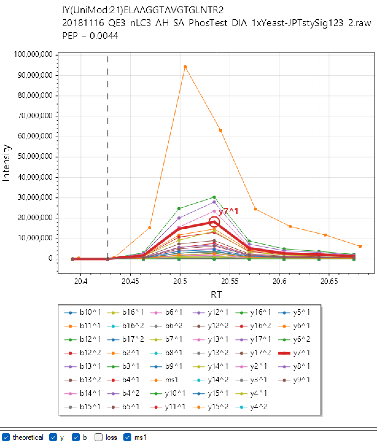
**Note**: The chromatograms extracted with "XICs" are saved in Apache .parquet format (file names end with '.xic.parquet') and can be readily accessed using R or Python. This can be sometimes convenient to prepare publication-ready figures (although can do that with Skyline or DIA-NN Viewer too), or even to set up automatic custom quality control for LC-MS performance.

Peptide & modification positions within a protein can be visualised using AlphaMap by the Mann lab https://github.com/MannLabs/alphamap.

### Automated pipelines
The pipeline window within the DIA-NN GUI allows to combine multiple analysis steps into pipelines. Each pipeline step is a set of settings as displayed by the GUI. One can add such steps to the pipeline, update existing steps, remove steps, move steps up/down in the pipeline, disable/enable (by double mouse-click) certain steps within the pipeline and save/load pipelines. Further, individual pipeline steps can be copy-pasted between different GUI tabs/windows (use Copy and Paste buttons for this). We always assemble all DIA-NN runs for a particular publication in a pipeline. One can also use DIA-NN pipelines to store configuration templates. When running the pipeline, each pipeline step is automatically saved as a separate one-step pipeline next to DIA-NN's main report.

The **Apply RegEx** functionality is useful primarily for migration of pipelines between different machines. This field allows to overwrite file paths in the pipeline using regular expression match-replace. The syntax is --regex "pattern to replace" "pattern to replace with",can use --regex multiple times. Use --ignore-case to ignore letter case when matching. For example, the command
```
--ignore-case --regex "diann.exe" "C:/DIA-NN/2.0/diann.exe" --regex "C:/Out" "C:/Out/2.0" --regex "C:\\Out" "C:/Out/2.0" --regex "mass-acc-cal 30" "mass-acc-cal 100"
```
changes the DIA-NN binary file location to that of a specific version, adjusts some of the file paths accordingly and adjusts the calibration mass accuracy setting if specified anywhere in the pipeline.

### Fine tuning prediction models

DIA-NN 2.0 introduces the ability to fine-tune its retention time (RT) and ion mobility (IM) prediction models. This is highly beneficial when looking for modifications on which DIA-NN's built-in models have not been trained on. Fine-tuning of the fragmentation predictor will also become available in the future.

Currently, the following modifications do no require any fine-tuning: UniMod:4 (C, carbamidomethylation), UniMod:35 (M, oxidation), UniMod:42 (N-term, acetylation), UniMod:21 (STY, phosphorylation). Fine-tuning may be somewhat beneficial for the following modifications: UniMod:121 (K, diglycine), UniMod:888 (N-term, K, mTRAQ), UniMod:255 (N-term, K, dimethyl). Fine-tuning is likely to signficantly boost detection of other modifications.

**Tuning**. To fine-tune DIA-NN's predictors, all you need is a spectral library (say, tune_lib.tsv, more on how to generate it yourself below) containing peptides bearing the modifications of interest. Type the following in **Additional options** and click **Run**:
```
--tune-lib tune_lib.tsv
--tune-rt
--tune-im
```
If the library does not contain ion mobility information, omit --tune-im. If some modifications are not recognised, declare them using --mod. Tuning usually takes several minutes. DIA-NN will produce three output files: tune_lib.dict.txt, tune_lib.tuned_rt.pt and tune_lib.tuned_im.pt. You can now generated predicted libraries using tuned models by supplying the following options to DIA-NN:
```
--tokens tune_lib.dict.txt
--rt-model tune_lib.tuned_rt.pt
--im-model tune_lib.tuned_im.pt
```

**Generating the tuning library**. If there is no suitable tuning library, one can always generate it directly from DIA data. For this, select one or several 'good' (typically, largest size) runs that are expected to contain peptides with the modifications of interest. These runs can also come from some public data set. Make a predicted library with DIA-NN by specifying all modifications of interest as variable or fixed (including those the predictor has already been trained on, if you expect to find them in the raw data). In vast majority of cases the max number of variable modifications can be set to 1-3, going higher is unlikely to be beneficial. Search the raw files using this predicted library in **Proteoforms** scoring mode, with **Generate spectral library** selected and **MBR** disabled. If the search space is large, the data comes from timsTOF, Orbitrap or Orbitrap Astral, and you would like to obtain the results quicker, set **Speed and RAM usage** to **Ultra-fast**. Optional: to optimise the performance, change the name of the output library and search the data again using --rt-window [X] and --im-window 0.2, where X is half of the gradient length (in minutes). Out of the two empirical libraries, choose the one with more modified peptides detected. Use this empirical library for fine-tuning.

If you use a tuning library that is not an empirical library generated by DIA-NN's lib-free search, and its RT & IM scales are significantly different from those produced by DIA-NN's predictors, it may be beneficial to adjust the RT & IM values in the tuning library to approximately match DIA-NN's (e.g. it's easy to do it if the tuning library contains some unmodified peptides, as those can be used for adjustment).

### PTMs and peptidoforms

DIA-NN GUI features built-in workflows (**Precursor ion generation** pane) for detecting methionine oxidation, N-terminal protein acetylation, phosphorylation and ubiquitination (via the detection of remnant -GG adducts on lysines). Other modificaitons can be declared using --var-mod or --fixed-mod in **Additional options**.

Distinguishing between peptidoforms bearing different sets of modifications is a non-trivial problem in DIA: without special peptidoform scoring the effective peptidoform FDR can be in the range 5-10% for library-free analyses. DIA-NN implements a statistical target-decoy approach for peptidoform scoring, which is enabled by the **Peptidoforms** **Scoring** mode (**Algorithm** pane) and is also activated automatically whenever a variable modification is declared, via the GUI settings or the --var-mod command. The resulting peptidoform q-values reflect DIA-NN's confidence in the correctness of the set of modifications reported for the peptide as well as the correctness of the amino acid sequence identified. These q-values, however, do not guarantee the absence of low mass shifts due to some amino acid substitutions or modifications such as deamidation (note that DDA does not guarantee this either). They are also not a replacement for dedicated channel-confidence scores, see [Multiplexing using plexDIA](#multiplexing-using-plexdia).

**Note**: for purely peptidomics applications, such as a typical phosphoproteomics experiment, we recommend the **Proteoforms** **Scoring** mode, see [GUI settings reference](#gui-settings-reference) for details.

Further, DIA-NN features an algorithm which reports PTM localisation confidence estimates (as posterior probabilities for correct localisation of all variable PTM sites on the peptide as well as scores for individual sites), included in the .parquet output report. When matrix output is enabled, DIA-NN also produces quantitative matrices for the PTM sites, calculated using the Top 1 method (experimental), that is the highest intensity among precursors with the site localised with the specified confidence (0.9 or 0.99, respectively) is used as the PTM quantity in the given run. Here, the sum of top 3 fragment intensities (ordered by their reference library intensities), multiplied by the precursor-specific normalisation factor, is used as the precursor intensity. One can also replace these with normalised MS1 apex intensities using --site-ms1-quant. The 'top 1' algorithm is used here as it is likely the most robust against outliers and mislocalisation errors. However, whether or not this is indeed the best option needs to be investigated, which is currently challenging due to the lack of benchmarks with known ground truth (precision in LFQbench-type experiments is not a good proxy, as it does not model the possibly differential regulation of sites on the same peptide). These matrices are currently not being produced when multiplexing is used (--channels), in this case please rely on the main report.

In general, when looking for PTMs, we recommend the following:

* Essential: the variable modifications you are looking for must be specified as variable (via the GUI checkboxes or the **Additional options**) both when generating an in silico predicted library and also when analysing the raw data using any predicted or empirical library.

* Settings for phosphorylation: max 3 variable modifications, max 1 missed cleavage, phosphorylation is the only variable modification specified, precursor charge range 2-3; to reduce RAM usage, make sure that the precursor mass range specified (when generating a predicted library) is not wider than the precursor mass range selected for MS/MS by the DIA method; to speed up processing when using a predicted library, first generate a DIA-based library from a subset of experiment runs (e.g. 10+ best runs) and then analyse the whole dataset using this DIA-based library with MBR disabled.

* When the above succeeds, also try max 2 missed cleavages.

* When looking for PTMs other than phosphorylation, in 95% of cases best to use max 1 to 3 variable modifications and max 1 missed cleavage.

* When not looking for PTMs, i.e. when the goal is relative protein quantification, enabling variable modifications typically does not yield higher proteomic depth. While it usually does not hurt either, it will make the processing slower.

Of note, when the ultimate goal is the identification of proteins, it is largely irrelevant if a modified peptide is misidentified, by being matched to a spectrum originating from a different peptidoform. Therefore, if the purpose of the experiment is to identify/quantify specific PTMs, amino acid substitutions or distinguish proteins with high sequence identity, then the **Peptidoforms** (or **Proteoforms**) scoring option is recommended. In all other cases peptidoform scoring is typically OK to use but not necessary, and will usually lead to a somewhat slower processing and a slight decrease in identification numbers when using MBR.

Does DIA-NN need to recognise modifications in the spectral library?

Yes. If unknown modifications are detected in the library, DIA-NN will print a warning listing those, and it is strongly recommended to declare them using --mod. Note that DIA-NN already recognises many common modifications and can also load the whole UniMod database, see the --full-unimod option.

### Multiplexing using plexDIA
We have developed plexDIA based on DIA-NN, a technology that allows to benefit from non-isobaric multiplexing (mTRAQ, dimethyl, SILAC) in combination with DIA. To analyse a plexDIA experiment, one needs an in silico predicted or empirical spectral library. DIA-NN then needs to be supplied with the following sets of commands, depending on the analysis scenario.

**Scenario 1**. The library is a regular label-free library (empirical or predicted), and multiplexing is achieved purely with isotopic labelling, i.e. without chemical labelling with tags such as mTRAQ or dimethyl. DIA-NN then needs the following options to be added to **Additional options**:
* --fixed-mod, to declare the base name for the channel labels and the associated amino acids
* --lib-fixed-mod, to in silico apply the modification declared with --fixed-mod to the library
* --channels, to declare the mass shifts for all the channels considered
* --original-mods, to prevent DIA-NN from converting the declared modifications to UniMod

Example for L/H SILAC labels on K and R:
```
--fixed-mod SILAC,0.0,KR,label
--lib-fixed-mod SILAC
--channels SILAC,L,KR,0:0; SILAC,H,KR,8.014199:10.008269
--original-mods
```
Note that in the above SILAC is declared as label, i.e. it is not supposed to change the retention time of the peptide. It is also a zero-mass label here, as it only serves to designate the amino acids that will be labelled. What the combination of --fixed-mod and --lib-fixed-mod does here is simply put (SILAC) after each K or R in the precursor id sequence, in the internal library representation used by DIA-NN. --channels then splits each library entry into two, one with masses 0 (K) and 0 (R) added upon each occurrence of K(SILAC) or R(SILAC) in the sequence, respectively, and another one with 8.014199 (K) and 10.008269 (R).

**Scenario 2**. The library is a regular label-free library (empirical or predicted), and multiplexing is achieved via chemical labelling with mTRAQ.

Scenario 2: Step 1. Label the library in silico with mTRAQ and run the deep learning predictor to adjust spectra/RTs/IMs. For this, run DIA-NN with the input library in the **Spectral library** field, an **Output library** specified, **Deep learning-based spectra, RTs and IMs prediction** enabled, list of raw data files empty and the following options in **Additional options**:
```
--fixed-mod mTRAQ,140.0949630177,nK
--lib-fixed-mod mTRAQ
--channels mTRAQ,0,nK,0:0; mTRAQ,4,nK,4.0070994:4.0070994;mTRAQ,8,nK,8.0141988132:8.0141988132
--original-mods
```
Use the .predicted.speclib file with the name corresponding to the **Output library** as the spectral library for the next step.

Scenario 2: Step 2. Run DIA-NN with the following options:
```
--fixed-mod mTRAQ,140.0949630177,nK
--channels mTRAQ,0,nK,0:0; mTRAQ,4,nK,4.0070994:4.0070994;mTRAQ,8,nK,8.0141988132:8.0141988132
--original-mods
```
Note that --lib-fixed-mod is no longer necessary as the library generated in Step 1 already contains (mTRAQ) at the N-terminus and lysines of each peptide.

**Scenario 3**. The library is a regular label-free library (empirical or predicted), and multiplexing is achieved via chemical labelling with a label other than mTRAQ. The reason this scenario is treated differently from Scenario 2 is that DIA-NN's in silico predictor has not been specifically trained for labels other than mTRAQ, and therefore an extra step to generate predictions is not necessary. Simply run DIA-NN as you would do in Scenario 1, except the --fixed-mod declaration will have a non-zero mass in this case and will not be a label. For example, for 5-channel dimethyl as described by [Thielert et al](https://doi.org/10.15252/msb.202211503):
```
‐‐fixed‐mod Dimethyl, 28.0313, nK
--lib-fixed-mod Dimethyl
‐‐channels Dimethyl,0,nK,0:0; Dimethyl,2,nK,2.0126:2.0126; Dimethyl,4,nK,4.0251:4.0251; Dimethyl,6,nK,6.0377:6.0377; Dimethyl,8,nK,8.0444:8.0444
--original-mods
```

**Scenario 4**. The library is an empirical DIA library generated by DIA-NN from a multiplexed DIA dataset. For example, this could be a library generated by DIA-NN in the first pass of MBR (and you'd like to reuse it to analyse the same or some other runs). The **Additional options** will then be the same as in Scenario 1, Scenario 2: Step 2 or Scenario 3, except (important!) --lib-fixed-mod must not be supplied.

**Scenario 5**. The sample is a light sample with heavy spike-in proteins or peptides, that is only a small proportion of precursors should feature multiple channels. In this case, start with two unlabelled spectral libraries, one for the whole proteome, another for the spike-ins. Make sure that the RT and IM scales in those are similar and fragmentation information is likewise comparable - this will be the case if the libraries are predicted by DIA-NN. Using [Editing spectral libraries](#editing-spectral-libraries) make sure that (i) the whole proteome library does not contain precursors corresponding to spike-in peptides and (ii) the spike-in library has appropriate channel family tags applied to the precursor/peptide names. Combine the libraries in DIA-NN and proceed as in **Scenario 3**, except omit --lib-fixed-mod.

**In all the scenarios above**, an extra option specifying the normalisation strategy must be included in **Additional options**. This can be either --channel-run-norm (pulsed SILAC, protein turnover) or -channel-spec-norm (multiplexing of independent samples).

**Output**. When analysing multiplexed data, the main report in .parquet format needs to be used for all downstream analyses. Note that PG.Q.Value and GG.Q.Value in the main report are channel-specific, when using multiplexing. The quantities PG.MaxLFQ, Genes.MaxLFQ and Genes.MaxLFQ.Unique are only channel-specific if (i) QuantUMS is used and (ii) either the report corresponds to the second pass of MBR or MBR is not used.

**Channel confidence**. DIA-NN estimates channel-confidence of identifications (expressed as Channel.Q.Value and PG.Q.Value) by searching an in silico generated 'decoy' channel and then comparing the numbers of identifications in this channel and cognate channels, at a given score threshold. The decoy channel generated is displayed by DIA-NN at the top of its log and can be overriden using --decoy-channel. Note that the channel confidence estimates obtained will be biased if the decoy channel turns out to be a poor model for the target channel-mismatched identifications. For example, in case of +0, +4 and +8 target channels, decoy channel +12 will result in conservative channel q-values if +8 is a carrier while +0 and +4 are single cells, and in optimistic channel q-values if +0 is the carrier. However, this fluctations in accuracy of channel confidence estimation would typically still allow for quality quantification with any reasonable (0.01-0.05) q-value filters.

**Note**: QuantUMS quality metrics provide independent control for channel confidence and can be used in addition or instead of channel-specific q-value filtering.

### Editing spectral libraries

This section summarises manipulations with spectral libraries that can be helpful for certain fancy experiments.

DIA-NN itself can:
* Convert any spectral library compatible with it to .parquet format. For this, specify the input library in **Spectral library** field and click **Run** (**Raw** field must be empty).
* Merge several .parquet or .tsv libraries, for this use multiple --lib commands in **Additional options**. Note the warnings printed by DIA-NN.
* Replace the spectra, RTs and IMs in the library with predicted ones using deep learning. Note --dl-no-fr, --dl-no-rt and --dl-no-im that allow to control what gets replaced.
* Apply fixed modifications to the library using --lib-fixed-mod. This changes peptide names and, if the modification has non-zero mass, also precursor and fragment masses.

Using R or Python, you can further:
* Edit .tsv or .parquet libraries in arbitrary way, including filtering, editing RTs and IMs, changing peptide sequences, adding 'faux' modifications (e.g. pasting '(SILAC)' after specific amino acids, to be later on used with --channels) and editing modification names, adding decoy peptides, marking fragments that should not be used for quantification, editing proteotypicity information for precursors, adjusting how proteins are annotated.
* Combine .tsv or .parquet libraries, here it is important to make sure that there are no duplicate precursors in the resulting library.

Note that if you edit and save a library in .parquet format to be used by DIA-NN, you need to ensure that (i) all floating point columns have the FLOAT parquet type and (ii) all integer or boolean columns have the INT64 parquet type. For this, when using R, it is best to load the table using read_parquet() function of the 'arrow' R package, with the argument as_data_frame=F. You can then apply most 'dplyr' package operations directly to this table, without using collect(). The edited table can be saved with write_parquet().

### Custom decoys

This section describes DIA-NN's ability to customise its decoy models, this is not needed for 99.9% of experiments.

This functionality is howerver essential for correct handling of data wherein a substantial proportion of peptides incorporates specific sequence patterns, and, to our knowledge, is a unique feature of DIA-NN. We further plan to expand the ways in which decoy generation is controlled, up to supporting fully-custom decoy generation algorithms, based on the feedback from the proteomics community.

DIA-NN implements two main approaches to decoy generation based on a target peptide: (i) shuffling of the residues using a particular algorithm and (ii) mutation of a single residue. DIA-NN has the following decoy generation parameters, which it will attempt to abide by whenever possible and will only ignore if it cannot generate the decoy otherwise:
* **--dg-keep-nterm [N]** do not change the first N residues, default N = 1
* **--dg-keep-cterm [N]** do not change the last N residues, default N = 1
* **--dg-min-shuffle [X]** aim for any fragment mass shift introduced by shuffling to exceed X in absolute value, default 5.0
* **--dg-min-mut [X]** aim for the precursor mass shift during mutation to be at least X in absolute value, default 15.0
* **--dg-max-mut [X]** aim for the precursor mass shift during mutation not to exceed X in absolute value, default 50.0

In particular, the options restricting N-term and C-term residue changes are essential in a situation when the target peptides are e.g. synthetic peptides that all share several N-term or C-term residues.

### Integration with other tools

This is a quick reference section for third-party software developers.

Starting with DIA-NN 2.0, it is possible to supply DIA-NN with decoy peptide queries in the spectral library (.parquet) along with the target peptides. This allows DIA-NN to use its MBR-optimised algorithm to correctly control FDR with empirical libraries generated by third-party software. For this, the third-party software needs to generate its libraries in DIA-NN-compatible .parquet format (i.e. include all the columns, the column 'Flags' can have 0 values). Ideally, the libraries should contain:
* A proportion of decoy peptides, corresponding the to q-value filtering applied when generating the library. DIA-NN will search these decoys in addition to the regular decoys it generates. Therefore, if the fraction of decoys is in the range of tens of percent (i.e. library FDR is >= 0.1), this will make the resulting DIA-NN's FDR estimates too conservative, which is fine for most experiments. Nevertheless, this ensures correct FDR control even with libraries filtered at >= 0.5 q-value.

* Q-values for all entries, target and decoy. While this is not essential to ensure FDR control provided decoys are included, DIA-NN's algorithms use these q-values to improve identification performance. In case decoys are not provided, including q-values may, in most cases, largely ensure correct FDR control by itself. It is, therefore, always recommended.

The numeric columns in DIA-NN's .parquet libraries are of types INT64 and FLOAT, other types should not be used.

For third-party downstream tools, it may be useful to have DIA-NN also export the decoy identifications using --report-decoys.

### Quantification

DIA-NN implements **Legacy (direct)** and **QuantUMS** quantification modes. The default QuantUMS (high-precision) is recommended in most cases. QuantUMS enables machine learning-optimised relative quantification of precursors and proteins, maximising precision while in many cases eliminating any ratio compression, see [Key publications](#key-publications). DIA-NN 2.0 has a much improved set of QuantUMS algorithms, compared to our original preprint.

Note that if you are analysing with an empirical library, you can quickly generate reports corresponding to different quantification modes with **Reuse .quant files**. This can also be done just for a subset of raw files, i.e. if you have analysed also blanks and now wish to exclude them.

We have observed that:
* QuantUMS performance is largely unchanged regardless of the experiment size, i.e. it is suitable for large experiments.

* QuantUMS works well also on experiments which include very different sample amounts (tested with 10x range across different samples). Note, however, that in this case the optimisation of QuantUMS parameters, automatically performed by DIA-NN, largely tunes the algorithm to quantify most accurately 'representative' identifications, i.e. if the experiment consists of 10 bulk runs and 10 single cell runs, optimisation will turn out to be optimal for bulk runs.

* QuantUMS has been tested with sub 2-minute to over 90 minute gradients and with both bulk and single cell-like samples.

* QuantUMS is particularly beneficial for Orbitrap Astral data due to the high quality of its MS1 spectra.

Below are some recommendations for the use of QuantUMS.

**High-accuracy**. Use the high-accuracy mode when you'd like to minimise the ratio compression at the cost of precision. Note that while it does a very good job at this in most cases, DIA-NN still cannot completely eliminate ratio compression for low-abundant precursors and proteins in challenging samples, e.g. when analysing nanogram amounts at 200-500 samples/day throughput. It is easy to see why: many precursors in such cases will not have a single high quality signal recorded.

**For large experiments**, train QuantUMS on a subset of runs (e.g. 10 to 100 representative runs with medium to high numbers of identified precursors) and then quantify the whole experiment by reusing the QuantUMS parameters. For this, first run QuantUMS on a subset of runs, you can do this by just selecting only those runs in **Raw** files window and checking **Reuse .quant files**. Alternatively, you can specifically instruct QuantUMS to train only on a range of raw files (by index, starting with 0) using --quant-train-runs first:last, e.g. --quant-train-runs 0:5 will perform training on identifications from the first 6 runs. A third option (not recommended) is to instruct DIA-NN to automatically select N runs (use N between 6 and 100) to train QuantUMS with --quant-sel-runs [N]. As output, you will see a list of quantificaton parameters printed in the log, e.g.
```
Quantification parameters: 0.330076, 0.123932, 1.03485, 0.324712, 0.241882, 0.271245, 0.161143, 0.0203897, 0.019745, 0.0728814, 0.0574469, 0.0620889, 0.206804, 0.0761579, 0.0977414, 0.0613432
```
You can then use those parameters and skip training on the whole (large) experiment by using --quant-params, e.g.
```
--quant-params 0.330076, 0.123932, 1.03485, 0.324712, 0.241882, 0.271245, 0.161143, 0.0203897, 0.019745, 0.0728814, 0.0574469, 0.0620889, 0.206804, 0.0761579, 0.0977414, 0.0613432
```
QuantUMS can be trained on replicate injections of the same sample: we have verified on a diverse set of LC-MS setups that such training results in near-optimal parameters even when trained on triplicates. Nevertheless, QuantUMS does require at least some degree of variation in the data. Even in replicate injections, some quantitative variation is always present due to flucations in instrument performance. Still, we recommend training QuantUMS on subsets of runs that include at least some non-replicates. This is no limitation, given that any 'real' experiment encompasses biological variation.

How optimal specific parameters are for a particular experiment depends on the LC-MS settings (gradient, acc/ramp times, acquisition scheme) and the general type of sample (e.g. whole-cell vs AP-MS). It is likely OK to even reuse QuantUMS parameters between experiments with the same LC-MS settings and general sample types, so long as the training is performed on data corresponding to the same or larger sample amounts and the 'instrument sensitivity' was at its highest when the training data were acquired. The opposite is not recommended.

**Filtering**. One of the benefits of QuantUMS is that it provides 'quality' metrics for each quantity it reports. We recommend using both Quantity.Quality and PG.MaxLFQ.Quality for filtering. In most cases, it makes sense to apply a relatively strict filter on the average quality metric for the analyte and much less strict filter on its run-specific quality metric. The average filter may increase numbers of DE analytes at a given FDR, as less analytes under consideration mean less strict multiple testing correction. The run-specific filter is best chosen to retain the vast majority of identifications, while eliminating the ones with very low quality quantities.

**Legacy mode** is to be used in the following cases:
* Always use the legacy mode when benchmarking LC-MS (settings). This is due to the fact that QuantUMS does not have the objective to minimise CV values, rather its goal is to achieve a good balance between precision and accuracy. This balance may differ significantly between different LC-MS settings, and using a single metric such as the median coefficient of variation (CV) reflects only part of this balance. Therefore, for experiments where QuantUMS simply decides to emphasise precision to a greater extent, CV values will appear better.

* You would like to use the top N protein quantities (normally not recommended) instead of the built-in QuantUMS MaxLFQ-like algorithm, QuantUMS precursor quantities are currently not inteded to be used for top N as QuantUMS is inherently a 'relative quantification' method, whereas top N effectively implies comparing quantities of different precursor ion species.

* For the same reason, use the legacy mode for IBAQ.

* In all the above (rare) cases where comparisons between quantities of different precursor species are performed (= absolute quantification is important) and the legacy mode is therefore appropriate, also consider just using the raw fragment quantities (at the apex), reported by DIA-NN when using --export-quant, e.g. summing the first 3 fragments may in some cases be better than using the legacy quantities. The normalisation factors calculated by DIA-NN in any mode can also be applied to the raw fragment quantities. Further, in all such scenarious you may want to use the top N approach (with N between 1 and 3) for any kind of precursor quantities aggregation (e.g. protein quant) rather than MaxLFQ (because if MaxLFQ were appropriate, would be better to use QuantUMS).

**Zero quantities**. Any of the quantities produced by DIA-NN may be equal to zero. The best interpretation here is that such quantities likely indicate an analyte with low concentration. If you would like to log-transform the data, can just replace those with NAs. We prefer to report zeroes rather than change the algorithm to output noise or NAs, as zeroes here provide information which may be of value for some downstream workflows.

**Synchro-PASEF**. When analysing Synchro-PASEF data, use --quant-tims-sum, which makes DIA-NN quantify each fragment in each DIA cycle by summing the signals recorded in all cognate frames within the cycle. While this is likely to provide fairly good performance, it is unknown if minor changes in the IM calibration of the instrument may add to batch effects when analysing using Synchro-PASEF, we will have certainty once benchmarks are available to assess this.

**Normalisation**. DIA-NN implements different normalisation modes. Normalisation can correct for different amounts of input material and sample losses. The RT-dependent normalisation further corrects for factors that differentially affect peptides depending on their hydrophobicity (reflected by their RT), i.e. some types of sample preparation losses, including desalting, as well as possibly also fluctations in the ion source performance. There are multiple examples of experiments where RT-dependent normalisation has a major positive effect on quantiative performance and no known cases where it is substantially detrimental.

**Limitations of normalisation**. In general, any kind of generic normalisation in proteomics only makes sense under the following assumption: when only considering 'biological' variability of interest, most of the peptides are not differentialy abundant, or the numbers of upregulated / downregulated (in comparison to experiment-wide averages) peptides in each sample are about the same. This assumption often is not strictly satisfied. Reasons range from non-linear dynamic range of the LC-MS to fundamental biological differences between the samples (e.g., ideally, different normalisation factors may need to be applied to cytosilic, plasma membrane or chromatin proteins, when comparing two single cells of different sizes). However, in many 'typical' proteomics experiments the normalisation algorithms implemented by DIA-NN work very well still. Nevertheless, it is recommended to not include blanks/failed runs in you quantitative analyses, i.e. if you are only processing blanks to figure out how many proteins are detectable in these, you can always process them separately with the emprical library produced by DIA-NN based on your experiment. Further, best to avoid a situation when the majority of precursors in a particular sample are not detectable in most other samples, e.g. not to include bulk runs in the quantitative analyses of single cell samples (but can absolutely use them to generate the empirical library).

**Disabling normalisation**. Given the above, there are scenarious (e.g. AP-MS, any kind of protein fractionation, time-series tracking isotopic label incorporation) when it may be desirable to apply custom normalisation that takes into account the nature of the experiment. In this case, we suggest either (i) disabling the normalisation in DIA-NN - you can still use MaxLFQ quantities in this case or (ii) keeping normalisation set to RT-dependent and applying custom normalisation on top of that, to benefit from DIA-NN correcting for any RT-dependent perturbations. The latter makes sense if there is still a considerable fraction of peptides that are shared between the samples.

**Fold-changes**. Given that normalisation is never 100% perfect, it is usually recommended to incorporate fold-change cutoffs in any differential expression (DE) analysis. These do not need to be particular large in magnitude, but should at least exceed the expected error in normalisation, e.g. when treating a cell line with drug compounds that have minor effects on the cells, even 10% fold-change cutoff may be appropriate. Fold-change cutoffs have also a further benefit of substantially reducing the FDR. Important: fold-change cutoffs must be applied after adjusting the p-values via multiple testing correction, not before.

**Detecting normalisation errors**. Errors in normalisation may be easy to identify. For example, the number of points with positive and negative fold-changes on a volcano plot should almost always be balanced. Indeed, one or several pathways may be upregulated in one condition compared to another, but if most pathways seem to be upregulated, it would mean most proteins are upregulated, implying that the dataset has not been correctly normalised. This does not apply to some special cases like AP-MS though.

A simple normalisation test can be carried in R or Python. For any two samples
* Calculate log2 fold-change of each analyte (precursor or protein) between the samples.
* Plot the histogram of the above log2 fold-changes.
* Indicate the median and half sample mode (use hsm() function of the modeest R package) on the histogram. Both these values should be close to 0.

**Raw fragment quantities**. DIA-NN has the --export-quant option, that appends theoretical as well as observed (per-run) information on the library fragment ions of a precursor (top 12 sorted by the reference intensity), such as the observed signal intensity (non-normalised) as well as a score reflecting fragment XIC quality. These are useful for connecting DIA-NN to downstream packages that require raw fragment quantities as well as for applications such as setting up MRM/PRM assays, as these data can be used to select fragments that are reliably detectable.

### Speed optimisation

This section focuses on factors that allow to increase the speed of processing and reduce RAM usage with large predicted spectral libraries.

**Analysing a subset of runs**. DIA-NN is very good at creating quality emprical spectral libraries from DIA data, and it does not need the whole experiment to do this. Although DIA-NN has been successfully used to search tens of thousands of runs lib-free, this is not really necessary in 99.9% of cases. In contrast, when processing large experiments, we recommend selecting 20 to 100 high quality runs (often selecting just the largest files works well) and create an empirical library from those (do not include blanks or failed runs here, they take by far the longest to process and are useless for library creation). This library can then be used to search the entire experiment (with **MBR** off). Further, if you have just acquired an experiment and want to quickly confirm that e.g. the runs did not fail and the mass calibration is OK, any suitable library can be used for this purpose, e.g. any public library or a DIA-based empirical library created based on a single run.

**Reducing the search space**. The time to search a file with a large library is approximately proportional to the size of the library. Therefore, we recommend to strictly follow the recommendations in this guide with respect to specifying variable modifications (i.e. only specify them if there are compelling reasons for this), at least for the first analysis. Once you have the data obtained using recommended settings, can see if including extra modifications improves identification numbers (in vast majority of cases it does not).

**Reducing RAM usage**. DIA-NN requires just under 0.5Gb RAM to store 1 million library precursors. That is a 3-million human tryptic digest library will require 1.5Gb RAM, while a 50-million library for phosphoproteomics will require about 25Gb of RAM. RAM is further used to store the raw data file that is being processed and for temporary storage of candidate PSMs. The requirements of the latter can be minimsed by adjusting **Speed and RAM usage**. There is currently a limit of max 1 billion precursor ions in the library, while DIA-NN is fine searching anything below that, provided it has enough RAM. If you are dealing with huge sequence databases, ubiquitous variable modifications or non-specific digests, resulting in libraries containing hundreds of millions precursors, it may make sense to split them and search separately. For example, a charge 2 length 8-13 (primary range for HLA peptides) non-specific human digest library (see --cut) is roughly 68 million precursors, i.e. including other charge states and the full length range here would not be manageable on regular desktop PCs. However, it is OK to search charge 1 and charge 2 separately, and then combine the resulting empirical libraries for the quantitative analysis. Similarly, predicted libraries can be also split based on the precursor m/z ranges. Further, imagine a metaproteomics experiment that is to be searched against 1000s of species. In this case, it may make sense to split the species into groups (e.g. by taxa or even randomly) and search those groups separately, looking, say, only for charge 2 precursors in 8-20 length range. This will allow to identify any confidently detected species (e.g. at least N proteins detected using proteotypic peptides) and then research only those in one go.

Note that during MBR search DIA-NN only stores .quant files on disk during the first pass, whereas during the second pass they are stored in-memory, increasing RAM usage for large experiments. MBR is just a convenience feature, for large experiments we recommend to reproduce it with a two-step procedure (create an empirical library and then analyse with this library) as described above.

**Speed and RAM usage**. This setting is useful on some instruments. Specifically, we have observed on a number of experiments that with **MBR** the peptidoform-confident identification numbers obtained in **Ultra-fast** mode can be the same or almost the same as in the **Optimal results** mode, while the **Ultra-fast** mode is often fold-change faster. This in particular applies to fairly heterogeneous samples (most real experiments). Therefore, on samples that take very long time to process (e.g. long-gradient slice/scanning methods on timsTOF or if searching with huge libraries) and require peptidoform confidence, an empirical library can indeed be generated using the **Ultra-fast** mode if you wish to obtain it quicker, we recommend trying this on Orbitrap, Orbitrap Astral and timsTOF data.

**RT window control**. During the analysis, DIA-NN automatically sets the width of the retention time (RT) window: this value provides guidance to DIA-NN's algorithms that make decisions at which points in the acquisition to look for each particular precursor ion. Reducing RT window makes the search faster but increases the chances of DIA-NN failing to identify precursors that have inaccurate reference RT values stored in the spectral library. For a further speed increase - when generating an empirical library - one can use --rt-window-mul 1.7 --rt-window-factor 100: if there are no modification-associated biases in the input library retention times (i.e. it's either an empirical library or a predicted library with models tuned, if necessary, as recommended in [Fine tuning prediction models](#fine-tuning-prediction-models)), this will likely result in comparable identification numbers. Before doing this, we recommend verifying on several acquisitions that reduced RT window does not result in a noticeable loss of identification numbers with particular sample type and LC-MS settings.

**Calibration speed**. DIA-NN will correctly process also raw data files with mass calibration that is off by up to ~100 ppm. DIA-NN also incorporates an algorithm that infers whether or not the data are well calibrated, and automatically tightens the mass tolerance used during the calibration state of the search, speeding it up. This algorithm may, in very rare cases, falsely misinterpret the MS/MS data (three such occurrances reported by the community before the release of DIA-NN 2.1.0). Therefore, given that in almost all cases it is known that the instrument is well calibrated, one can use --mass-acc-cal 25 to fix the calibration mass tolerance to 25 ppm.

**Optimising RAM access on Linux**. To possibly increase performance on some systems, one can use mimalloc with dynamic override as described here https://github.com/microsoft/mimalloc for all steps except predicted library generation. However, in most cases this will have no effect. When running multiple DIA-NN instances in parallel, one per NUMA node, one may want to check if assigning a specific node to each instance with numactl (--cpunodebind and --preferred options, along with the --privileged Docker option when running as a Docker container) results in a speed improvement on the specific system.

### Incremental processing

This sections focuses on the ways to handle large experiments wherein raw data is being gradually added over a long period of time.

**Fast reanalysis**. DIA-NN supports adding runs to the experiment and analysing them quickly, without having to reanalyse the whole experiment. For this, first create an empirical spectral library as recommended in the **[Speed optimisation](#speed-optimisation)** section above. Analyse each incoming batch of runs separately with this library, make sure that the mass accuracies and the scan window are fixed to specific values. If using QuantUMS, train it on a subset of runs as described in [Quantification](#quantification). Analyse all the runs acquired so far while specifying **Reuse .quant files** - this will only perform the cross-run steps of the analysis.

**Adding runs without changing any quantities**. If this is a requirement, we recommend, in addition to the above, to use the **Legacy (direct)** quantification mode as well as pass --no-maxlfq and --export-quant to DIA-NN. You then obtain raw fragment quantities (as well as raw MS1 quantities that are present regardless of the above settings). Below are some recommendations for obtaining the best quantitative performance (requires R or Python) that roughly correspond to the quantification apporach used by DIA-NN in legacy mode.
* When you generate your empirical library, select top 3 fragments for each precursor, based on their average scores (also reported when using --export-quant) across the respective (**reference**) runs. Further, when generating a library, select a set of least variable precursors (e.g. aim to select 40% of all precursors) and calculate their average log2 quantities.

* When processing DIA-NN output for all runs, calculate non-normalised precursor quantities by summing the selected fragments, replace zero quantities with NA values (important: always use the same logarithm base throughout the script, it's very easy to get incorrect results by accidentally mixing natural logarithms with log2).

* For each run, calculate the log2 fold-change for each detected precursor with respect to the average log2 levels as recorded across reference runs. Split the retention time range in bins (e.g. 100 bins, aim for 200+ precursors detected per bin). For each bin, calculate either the median or the half sample mode (hsm() function of the modeest package) of those log2 fold-changes of the selected precursors that fall within the bin or the adjacent bins, this value is the normalisation factor for the bin. Interpolate the normalisation factor, to calculate it for every RT. Apply this factor to all precursor identifications depending on their RT. Repeat the procedure with 2x-4x less bins (i.e. larger bins), eventually obtaining 'normalised' precursor quantities.

* For each batch (here 'batch' refers to any factor that may introduce technical batch effects, e.g. 384 plate used to grow cells), for each precursor, determine a batch correction factor to be applied to its normalised values. For example, if in **reference runs** a particular precursor was showing 2x higher intensity in HeLa QC injections than in the batch under consideration, then the batch correction factor for this precursor would be equal to 2.0. Alternatively, can calculate batch correction factors also based on average (log-scale) levels of a particular precursor across the biological samples of interest, provided those are appropriately randomised. Apply these correction factors to the normalised precursor quantities.

* Use the top 1 method to quantify proteins, i.e. in each run the normalised protein quantity is by definition the maximum of the normalised quantities of matching precursors detected at <= 0.01 q-value in this run. May apply protein-level normalisation on top of these, similarly to the precursor-level normalisation, except there is no need to perform RT-binning.

### Basics of DIA data analysis

This section is a short introduction to DIA proteomics data analysis without assuming any previous background in proteomics.

**Raw data**. Each raw DIA acquisition is a collection of MS1 and MS2 (also called MS/MS) spectra. Typically, a single MS1 spectrum and multiple MS2 spectra are recorded in each DIA cycle, and the duration of the cycle (0.3s - 3s) is such as to allow for multiple DIA cycles during the elution of a typical peptide from the LC system. Each MS1 spectrum represents the m/z values (mass over charge) and signal intensity values for the ions generated by the ion source ('precursor' ions), whereas each MS2 spectrum comprises m/z values for their fragments, generated in the collision cells of the mass spectrometer. Typically, to reduce the complexity of MS2 spectra, a mass filter (usually called 'Q1 quadrupole') is used to isolate a particular mass range of precursor ions for fragmentation, e.g. 500-520 m/z or 500.5-501.5 m/z - called 'mass isolation window' or 'selection window' (typically 2 m/z - 50 m/z in DIA).

**Spectral libraries**. In order to quantify peptides and proteins from the raw data, DIA-NN needs to know which peptides to look for. For example, DIA-NN can be provided with a sequence database (e.g. a reference UniProt proteome in uncompressed .fasta format) as input. DIA-NN can then generate 'precursor ion queries' based on the sequence database. That is, DIA-NN in silico digests the database using the provided enzyme specificity (e.g. trypsin), applies fixed (always present) and variable (may or may not be present) modifications to the resulting peptides and generates 'precursors' as peptides at a particular charge state. Now, given this set of precursors, it's possible to generate all theoretical fragment ions (which are peptide N-terminal and C-terminal fragments produced by the breakage at the peptide bond) and search the raw data for occurances of those. However, raw data search turns out to be much more efficient if the theoretical properties of individual peptides/precursors are predicted with deep learning, i.e. the retention time (RT; term used to refer to elution time of the peptide from the liquid chromatography (LC) system), the ion mobility (IM) and the fragmentation pattern. DIA-NN can do this, with the result being an in silico predicted 'spectral library'. In general, the term 'spectral library' refers to a set of known spectra, retention times and potentially also ion mobility values for selected precursor ions.

Spectral libraries can differ based on how they are generated. What is described above is a predicted spectral library, which may contain millions of entries (e.g. a spectral library based on human UniProt proteome tryptic digest contains about 5 million precursors with charges 1 to 4). Further, spectral libraries can be empirically generated, i.e. contain only precursors observed in a particular experiment. A common strategy has been to perform offline fractionation of a peptide sample (e.g. whole-cell tryptic digest) with subsequent analysis of each of the fractions by LC-MS and the generation of a spectral library comprising the set of confidently identified precursors. This has been traditionally done with DDA, but also works with DIA. In fact, DIA-NN is capable of generating a library from the analysis of any DIA data. That is, one can take a predicted library, search some raw data with it and obtain as a result a much smaller empirical DIA-based library. This library can then be used for a quantitative analysis of the same DIA experiment but also other DIA experiments. The present guide contains detailed explanations of possible workflows based on DIA-NN and guidance on their use.

**FDR control**. DIA data analysis produces a list of precursors and proteins identified in each of the samples of the experiment. Here 'identified' means that the software expects a particular proportion of those identifications, e.g. 1%, to be false, while the rest, e.g. 99%, are expected to be true. The way DIA-NN does this is by creating a list of likely PSMs (precursor-spectrum matches) and then narrowing it down to only retain PSMs passing certain quality thresholds. This kind of confidence in PSMs is represented by so-called q-values, i.e. 0.01 q-value corresponds to 1% FDR (false-discovery rate). Here it is important to emphasise that if DIA-NN does not report a particular precursor or protein as identified, it does not mean that it is necessarily missing from the sample. Rather this only means that the respective precursor or protein is likely to be relatively low-abundant.

DIA-NN supports both run-specific and global FDR control. Unlike run-specific q-values, global q-values allow to achieve confidence that a particular precursor or protein was correctly identified in at least one mass spectrometry run of the experiment. This is important in particular for large experiments. Indeed, if with each run in the experiment 1% of the identifications are just random noise (at 0.01 run-specific q-value), and all precursors in the library (e.g. 5 million) are equally likely to be falsely identified, then with a large enough experiment all library precursors will eventually be reported as identified in at least one run. Filtering based on global q-values allows to make sure that this does not happen. It also allows DIA-NN to generate high-quality empirical spectral libraries from arbitrary large DIA experiments.

**Quantification**. Each identified precursor or protein can be quantified in DIA, as all the signals recorded in DIA are quantitative. Here 'quantification' refers to 'relative quantification', wherein the levels of a precursor or a protein can be compared between different runs of the experiment, and hence also between different biological conditions of interest. Importantly, the reported quantities are not expected to be comparable between distinct precursors or between distinct proteins. This limitation originates from the fact that ionisation efficiency of different peptides can vary by orders of magnitude, depending on the peptide sequence. That being said, 'absolute quantification' is possible with DIA. Same as in SRM/PRM, isotopically-labelled peptides can be spiked into the sample in known molar amounts, to quantify their endogenous unlabelled counterparts, using the fact that the ionisation efficiency does not depend on the isotopic composition. Alternatively, absolute quantities of proteins can be estimated with approaches such as IBAQ, although such estimates tend to be of fairly low precision.

Of note, by default DIA-NN reports 'normalised' quantities. This means it makes the best effort to correct for any kind of technical variation in the data that affects all precursors at the same time, such as any kind of pipetting imprecision in sample preparation or different amounts of starting sample material. Indeed, consider a situation when one compares the proteomes of two single cells. If one cell is twice larger, then without normalisation almost every protein will appear differentially expressed. However, such a conclusion is of hardly any biological interest, hence the need for normalisation. Nevertheless, DIA-NN can also provide raw non-normalised intensities, if these are needed given a particular experiment design.

**Notes on terminology**:
- 'peptide' can be used to refer also to precursor ions;
- 'FDR' can be used interchangeably with 'q-value', although these are, strictly-speaking, not equivalent;
- the term 'library-free analysis' usually refers to using DIA-NN with a predicted spectral library generated from the whole sequence database, that is without an empirical library.

**Use of R or Python**. We have designed DIA-NN in such a way that the whole workflow requires zero bioinformatics expertise, i.e. indeed all downstream statistical analyses and visualisation can be carried out using MS Excel or similar software as well as dedicated visual tools for proteomics data analysis. However, once you have analysed your data and are now preparing a publication, we do recommend learning some basics of data analysis in R. R is a 'programming language' which nevertheless is very easy to master as coding data processing in R is in a sense similar to formulating a series of bullet points in natural language. Based on experience of a number of colleagues who have had zero prior programming experience, it takes between a day and a week to master R to a level which allows to confidently work with proteomics data (you only need very basics). Indeed, it may take one an hour or so to make several plots in Excel, and only several minutes in R. But most importantly, if you need to adjust your plots or the underlying data, it may be again just minutes in R (change a couple of lines of code and re-run the script), overall it greatly simplifies any kind of work with proteomics data and eventually saves a lot of time. We recommend starting here https://education.rstudio.com/learn/beginner/. This particular section https://r4ds.had.co.nz/data-visualisation.html nicely demonstrates how easy it is to create informative diagrams in R with just one or two lines of code.

### GUI settings reference

Input

* **Convert to .dia** Convert the selected raw files to DIA-NN's .dia format, for faster subsequent processing, and save them either to the same folder as the respective source raw files or to **Temp/.dia dir** (**Output** pane), if the latter is specified. Conversion is recommended for Sciex files, typically makes little difference for Thermo files and is not recommended for Bruker files.
* **Spectral library** specify the spectral library.
* **Add FASTA** add one or more FASTA files. FASTA files must always be specified if **Protein inference** is not disabled (see below) or you would like to obtain protein-matched phosphosite information. The only reason not to specify FASTA files is a situation when you are using an empirical library generated with the use of a different FASTA database that is not available, and in such case specifying FASTA files will overwrite the annotation of protein sequence IDs in the library, potentially replacing protein names, genes and descriptions.
* **Reannotate** option allows to reannotate the spectral library with protein information from the FASTA database, using the specified digest specificity.
* **Contaminants** Adds common contaminants from the Cambridge Centre for Proteomics (CCP) database and automatically excludes them from quantification, see the description of the --cont-quant-exclude option. This option applies when generating a predicted spectral library from a FASTA database or analysing using such a library, if it was generated with **Contaminants** enabled.

Precursor ion generation

* **FASTA digest** instructs DIA-NN to in silico digest the sequence database and apply specified modifications (see below), to generate a predicted spectral library in silico. This option must be unchecked when analysing raw data.
* **Deep learning-based spectra, RTs and IMs prediction** instructs DIA-NN to perform deep learning-based prediction of spectra, retention times and ion mobility values. This allows not only to make in silico spectral libraries from sequence databases, but also to replace spectra/RTs/IMs in existing libraries with predicted values. This option must not be used together with raw data analysis, i.e. in silico predicted library generation must be done in a separate step.
* **Protease** use pre-configured digest specificity, can be customised using the --cut command. Only affects FASTA digest or reannotation.
* **Missed cleavages** set the maximum number of missed cleavages allowed. Only affects FASTA digest. Increases the search space and hence the analysis time, setting to 1 is almost always the best, in some cases 2 may be beneficial, higher values are likely detrimental.
* **Maximum number of variable modifications** sets the maximum total number of occupied variable modification sites per peptide, only affects FASTA digest. Reasonable values are usually in 1 to 3 range, setting to 4 or higher is almost always detrimental. Substantially increases the search space and hence the analysis time and RAM usage, may have some detrimental effects on the identification numbers if set too high. Only specify variable modifications if (i) a substantial proportion of detectable peptides is expected to bear the specified number of variable modifications or (ii) you are interested in the biology of a specific modification.
* **N-term M excision** consider the removal of the protein N-term methionine as a variable modification. Always use this when the database contains actual proteins, rather than just a set of individual peptides.
* **C carbimidomethylation** declares C(cam) as a fixed modification, see --fixed-mod.
* **Ox(M), Ac(N-term), Phospho, K-GG** - these options declare the respective modifications as variable, see --var-mod. In case of **Phospho** declaration applies to S, T and Y. In case of K-GG, instructs DIA-NN to not add diglycine on C-terminal lysine of non-protein-C-term peptides, as enzymes such as trypsin or LysC would not cut after a lysine with a diglycine adduct, see --no-cut-after-mod.
* **Precursor and fragment ranges** allow to limit which precursors and fragments can be included in the predicted spectral library during FASTA digest. Important: always set minimum precursor charge to 2 when generating predicted libraries for searching timsTOF data, unless the acquisition scheme specifically selects charge 1 precursors for fragmentation (only the case for certain applications, such as immunopeptidomics).

Output

* **Reuse .quant files** reuse IDs/quantification information from a previous analysis, see [Output](#output)
* **Quantities matrices** generate text tables with quantities, see [Output](#output)
* **XICs** generate extracted ion chromatograms for DIA-NN Viewer, see [Visualisation](#visualisation)
* **Temp/.dia dir** specify where .quant files or converted .dia files will be saved, see [Output](#output)
* **Generate spectral library** generate either a predicted library (library name specified by **Predicted library** below), if no raw data specified, or an empirical DIA-based library (library name specified by **Output library** below), if analysing raw data.
* **Generate Prosit input** when performing FASTA digest, create an output file that can be used as input for the Prosit tool. This is helful if you are interested in testing Prosit, however not needed for DIA-NN itself.
* **Threads** suggest the number of CPU threads for DIA-NN to use. DIA-NN may not scale well beyond 64 threads.
* **Precursor FDR (%)** set the precursor q-value filtering to be applied to the main output report and the empirical spectral library to be generated. Normally should be kept at 1%, increasing up to 5% may be be helpful if the identification numbers are very low. Increasing beyond 5% is not recommended. Decreasing below 1% may result in worse protein quantification and is also not recommended.
* **PDF** generate per-file and experiment-wide PDF reports with some QC metrics and trends.

Algorithm

* **Mass Accuracy** set the MS2 mass tolerance (in ppm), see [Changing default settings](#changing-default-settings). Note: there is a view that setting this to very low values may improve quantification. This is not correct, setting to values that are too low may in fact result in a significant loss of quantitative precision.

* **Mass Accuracy MS1** set the MS1 mass tolerance (in ppm), see [Changing default settings](#changing-default-settings).

* **Scan window** sets the scan window radius to a specific value. Ideally, should be approximately equal to the average number of data points per peak, see [Changing default settings](#changing-default-settings).

* **MBR** activates a mode in DIA-NN which we call 'match-between-runs'. Note that the algorithm is fundamentally different from MBR in some DDA software. In MBR mode, DIA-NN does two passes over the data. During the first pass, it creates an empirical spectral library from the data. During the second pass, it reanalyses the experiment with this empirical library, which may result in much improved identification numbers, data completeness and quantification accuracy. Always use MBR for quantitative analyses (as opposed to analyses just aimed at creating an empirical library), unless you are analysing with a DIA-based empirical library (in that case do not use MBR). If you are analysing with a project-specific DDA-based library, it may make sense to compare results with and without MBR. For this, analyse first with MBR. You will get both the final MBR report as well as a report based on the first MBR pass (named main_report_name-first-pass.parquet). Compare the identification numbers and data completeness in the two reports. If you decide the performance is higher for the first pass, just uncheck **MBR**, select **Reuse .quant files**, change the main output file name and click **Run**.

MBR is great for small-scale and medium-scale experiments. However, in case of large-scale experiments, one does not need the whole dataset to create a high-quality empirical library. In such cases, we recommend selecting 20 to 100 high quality runs (often selecting just the largest files works well) and create an empirical library from those (that being said, it is perfectly fine to create a library from just a single run as well as thousands of runs). You can then use this library for the analysis of any experiments with matching sample types. Another scenario where one may want to create an empirical library in a separate step is when analysing single-cell data. In this case, it is a good idea to create a library based on some bulk sample runs or runs acquired based on 4-20 cells per sample. Finally, creating an empirical library in a separate step just offers more flexibility. For example, one can then quickly try different quantification modes using **Reuse .quant files**. Note: do not use empirical libraries generated based on non-timsTOF experiments to analyse timsTOF data. The opposite is fine.

* **Unrelated runs** determine mass accuracies and scan window, if automatic, independently for different runs, see [Changing default settings](#changing-default-settings).

* **Protein inference** whether or not to 'infer' proteins present in the sample using a maximum parsimony algorithm. When set to "Off", protein groups from the spectral library are used - this makes sense if protein inference has already been performed during library generation. In all other cases keep protein inference enabled. Protein inference basically means that DIA-NN creates a 'protein group' for each precursor, which is a subset of all protein IDs matched to the precursor. DIA-NN does so aiming to (i) reduce as much as possible the list of proteins matched to the precursor, using any hint it can to prioritise proteins that are more likely to explain the precursor while (ii) ensuring that if two identified precursors are matched to distinct protein groups, then these protein groups do not contain shared proteins. Note that maximum parsimony approaches for protein grouping can result in the following. If precursor X is annotated with proteins A and B, Y - B and C, Z - A and C, then the restriction (ii) will inevitably lead to a situation when protein groups for some of the precursors are missing proteins that could be present in the sample, e.g. groups could be A for X, and C for both Y and Z, whereas protein B is not included in any group. Therefore, the best practice is usually to either (i) use protein groups for any kind of system-scale analysis but manually confirm the differential regulation of proteotypic (i.e. specific to the protein) peptides for specific proteins of particular interest or (ii) rely only on proteotypic peptides.

* **Scoring** specifies the type of identification confidence. DIA-NN assigns q-values to target precursors based on how well the respective PSMs score in comparison to in silico generated decoy precursors, i.e. 'faux' peptides not expected to be present in the sample generated by DIA-NN via shuffling or mutation of residues within target peptides, with the respective adjustment of the precursor and fragment masses. The way these decoy peptides are generated is the fundamental factor behind the interpretation of q-values obtained. Please also see [Custom decoys](#custom-decoys).

In the **Generic** mode, DIA-NN rearranges part of the peptide sequence, aiming to change almost all of the theoretical fragment masses. Since there are no amino acid mutations generated, the precursor mass stays the same (there may be some rare exceptions when DIA-NN cannot sufficiently shuffle the sequence and uses amino acid mutations also in this mode). This is how DIA proteomic data analysis has been traditionally performed: this strategy maximises the numbers of identified proteins. The q-values in this case reflect the confidence that a precursor was correctly matched to a spectrum that has either originated from the same ion species or from an ion species that shares a signficant number of fragment ions (this is a very complex subject, here 'significant' cannot be defined precisely), has the m/z value that falls within the same DIA window, similar enough retention time and (if applicable) similar enough ion mobility. This kind of confidence is sufficient for most experiments of the 'typical proteomics experiment' type. We therefore recommend using this mode if you are interested in protein-level quantification and do not need to confidently distinguish between paralogues or orthologues.

In the **Proteoforms** mode (new in **DIA-NN 2.0**), DIA-NN generates decoys by mutating a single residue within each target precursor. This usually results in decoys that share a number of fragment ion masses with the respective targets but differ in the precursor mass. This decoy model is perfect for achieving confidence in the correct assignment of PTMs and correct identification of amino acid substitutions. The resulting q-values can be interpreted as confidence that the spectrum to which a precursor is matched has originated from an ion that not just shares a signficant number of fragment ion masses with it, but also has the same m/z value (within the applicable mass tolerances). Note the two limitations of this strategy (these apply to DDA data too). First, it is not effective in correctly identifying residue localisation within the peptide: phosphate localisation, for example, requires a separate scoring module in DIA-NN. Second, if, for example, the variable modification of interest has the mass equal to several heavy carbon mass deltas (i.e. = n * 1.003355, where n = 1,2,3,4), then the chance of misidnetifying those peptides will be increased even in the Proteoforms mode. This is the reason why DIA-NN has a separate scoring module for channel-specific confidence in plexDIA data analysis. In general, the **Proteoforms** mode is recommended for (i) most peptidomics applications, (ii) all applications where it's important to distinguish between close paralogues or orthologues and (iii) any data wherein the difference between identification numbers in Generic and Proteoforms modes is negligible, which is the case for many Orbitrap Astral and timsTOF datasets, especially those acquired with longer gradients.

In the **Peptidoforms** mode, DIA-NN's main q-values correspond to the regular decoy model, same as in the **Generic** mode, while extra peptidoform q-values provide peptidoform confidence levels. This mode is recommended if (i) you need global (i.e. experiment-wide) peptidoform confidence for some peptides but would also like to maximise the numbers of detected proteins, and (ii) the **Proteoforms** mode results in a non-negligible reduction of protein identification numbers on the dataset of interest. Note that since two types of q-value filtering are applied simultaneously in **Peptidoforms** mode, the numbers of precursors with peptidoforms q-values below 0.01 will typically be slightly lower than the numbers of precursors with q-values below 0.01 in the **Proteoforms** mode (for the first MBR pass), while the actual peptidoform FDR will also be slightly lower. The above differences are typically negligible.

**Note**: given that protein inference and protein q-value calculation are performed using all identified precursors, it is only the **Proteoforms** mode that can be used to reliably distinguish paralogue/orthologue proteins originating due to amino acid substitutions, hence the name for this mode.

* **Machine learn

ecosyste.ms

Data

Tools

Indexes

Applications

Experiments

Awesome

https://github.com/vdemichev/DiaNN

Awesome Lists containing this project

README

DIA-NN