Ecosyste.ms: Awesome
An open API service indexing awesome lists of open source software.
https://github.com/wizzat/distribution
Short, simple, direct scripts for creating ASCII graphical histograms in the terminal.
https://github.com/wizzat/distribution
Last synced: 7 days ago
JSON representation
Short, simple, direct scripts for creating ASCII graphical histograms in the terminal.
- Host: GitHub
- URL: https://github.com/wizzat/distribution
- Owner: wizzat
- License: gpl-2.0
- Created: 2012-08-14T20:01:34.000Z (about 12 years ago)
- Default Branch: master
- Last Pushed: 2021-10-06T01:43:32.000Z (about 3 years ago)
- Last Synced: 2024-08-02T16:54:07.102Z (3 months ago)
- Language: Python
- Size: 249 KB
- Stars: 453
- Watchers: 25
- Forks: 23
- Open Issues: 3
-
Metadata Files:
- Readme: README.md
- License: LICENSE.md
Awesome Lists containing this project
README
distribution
============
Short, simple, direct scripts for creating character-based graphs in a
command terminal. Status: stable. Features added very rarely.
Purpose
=======
To generate graphs directly in the (ASCII-based) terminal. Most common use-case:
if you type `long | list | of | commands | sort | uniq -c | sort -rn` in the terminal,
then you could replace the final `| sort | uniq -c | sort -rn` with `| distribution` and
very likely be happier with what you see.
The tool is mis-named. It was originally for generating histograms (a distribution
of the frequency of input tokens) but it has since been expanded to generate
time-series graphs (or, in fact, graphs with any arbitrary "x-axis") as well.
At first, there will be only two scripts, the originals written in Perl and
Python by Tim Ellis. Any other versions people are willing to create will be placed
here. The next likely candidate language is C++.
There are a few typical use cases for graphs in a terminal as we'll lay out here:
## Tokenize and Graph
A stream of ASCII bytes, tokenize it, tally the matching tokens, and graph
the result. For this example, assume "file" is a list of words with one word
per line, so passing it to "xargs" makes it all-one-line.
```
$ cat file | xargs #put all words on one line
this is an arbitrary stream of tokens. this will be graphed with tokens pulled out. this is the first use case.
$ cat file | xargs | distribution --tokenize=word --match=word --size=small -v
tokens/lines examined: 25
tokens/lines matched: 21
histogram keys: 17
runtime: 8.00ms
Key|Ct (Pct) Histogram
this|3 (14.29%) -----------------------------------------------------------------------o
is|2 (9.52%) ---------------------------------------o
tokens|2 (9.52%) ---------------------------------------o
graphed|1 (4.76%) -------o
will|1 (4.76%) -------o
```
## Aggregate and Graph
An already-tokenised input, one-per-line, tally and graph them.
```
$ cat file | distribution -s=small -v
tokens/lines examined: 21
tokens/lines matched: 21
histogram keys: 18
runtime: 14.00ms
Key|Ct (Pct) Histogram
this|3 (14.29%) -----------------------------------------------------------------------o
is|2 (9.52%) ---------------------------------------o
graphed|1 (4.76%) -------o
be|1 (4.76%) -------o
```
## Graph Already-Aggregated/Counted Tokens
A list of tallies + tokens, one-per-line. Create a graph with labels. This matches
the typical output of several Unix commands such as "du."
```
$ du -s /etc/*/ 2>/dev/null | distribution -g -v
tokens/lines examined: 107
tokens/lines matched: 5,176
histogram keys: 107
runtime: 2.00ms
Key|Ct (Pct) Histogram
/etc/ssl/|920 (17.77%) -------------------------------------------
/etc/init.d/|396 (7.65%) -------------------
/etc/apt/|284 (5.49%) -------------
/etc/nagios-plugins/|224 (4.33%) -----------
/etc/cis/|188 (3.63%) ---------
/etc/nagios/|180 (3.48%) ---------
/etc/fonts/|172 (3.32%) --------
/etc/ssh/|172 (3.32%) --------
/etc/default/|164 (3.17%) --------
/etc/console-setup/|132 (2.55%) -------
```
## Graph a List of Integers
A list of tallies only. Create a graph without labels. This is typical if you just
have a stream of numbers and wonder what they look like. The `--numonly` switch is
used to toggle this behaviour.
There is a different project: https://github.com/holman/spark that will produce
simpler, more-compact graphs. By contrast, this project will produce rather
lengthy and verbose graphs with far more resolution, which you may prefer.
Features
========
0. Configurable colourised output.
1. rcfile for your own preferred default commandline options.
2. Full Perl tokenising and regexp matching.
3. Partial-width Unicode characters for high-resolution charts.
4. Configurable chart sizes including "fill up my whole screen."
Installation
============
If you use homebrew, `brew install distribution` should do the trick, although
if you already have Perl or Python installed, you can simply download the file
and put it into your path.
To put the script into your homedir on the machine you plan to run the script:
```
$ wget https://raw.githubusercontent.com/philovivero/distribution/master/distribution.py
$ sudo mv distribution.py /usr/local/bin/distribution
$ alias worddist="distribution -t=word"
```
It is fine to place the script anywhere in your `$PATH`. The worddist alias is
useful for asking the script to tokenize the input for you eg `ls -alR | worddist`.
Options
=======
```
--keys=K periodically prune hash to K keys (default 5000)
--char=C character(s) to use for histogram character, some substitutions follow:
pl Use 1/3-width unicode partial lines to simulate 3x actual terminal width
pb Use 1/8-width unicode partial blocks to simulate 8x actual terminal width
ba (▬) Bar
bl (Ξ) Building
em (—) Emdash
me (⋯) Mid-Elipses
di (♦) Diamond
dt (•) Dot
sq (□) Square
--color colourise the output
--graph[=G] input is already key/value pairs. vk is default:
kv input is ordered key then value
vk input is ordered value then key
--height=N height of histogram, headers non-inclusive, overrides --size
--help get help
--logarithmic logarithmic graph
--match=RE only match lines (or tokens) that match this regexp, some substitutions follow:
word ^[A-Z,a-z]+$ - tokens/lines must be entirely alphabetic
num ^\d+$ - tokens/lines must be entirely numeric
--numonly[=N] input is numerics, simply graph values without labels
actual input is just values (default - abs, absolute are synonymous to actual)
diff input monotonically-increasing, graph differences (of 2nd and later values)
--palette=P comma-separated list of ANSI colour values for portions of the output
in this order: regular, key, count, percent, graph. implies --color.
--rcfile=F use this rcfile instead of $HOME/.distributionrc - must be first argument!
--size=S size of histogram, can abbreviate to single character, overridden by --width/--height
small 40x10
medium 80x20
large 120x30
full terminal width x terminal height (approximately)
--tokenize=RE split input on regexp RE and make histogram of all resulting tokens
word [^\w] - split on non-word characters like colons, brackets, commas, etc
white \s - split on whitespace
--width=N width of the histogram report, N characters, overrides --size
--verbose be verbose
```
Syslog Analysis Example
=======================
You can grab out parts of your syslog ask the script to tokenize on non-word
delimiters, then only match words. The verbosity gives you some stats as it
works and right before it prints the histogram.
```
$ zcat /var/log/syslog*gz \
| awk '{print $5" "$6}' \
| distribution --tokenize=word --match=word --height=10 --verbose --char=o
tokens/lines examined: 16,645
tokens/lines matched: 5,843
histogram keys: 92
runtime: 10.75ms
Val |Ct (Pct) Histogram
ntop |1818 (31.11%) ooooooooooooooooooooooooooooooooooooooooooooooooooooooo
WARNING |1619 (27.71%) ooooooooooooooooooooooooooooooooooooooooooooooooo
kernel |1146 (19.61%) ooooooooooooooooooooooooooooooooooo
CRON |153 (2.62%) ooooo
root |147 (2.52%) ooooo
message |99 (1.69%) ooo
last |99 (1.69%) ooo
ntpd |99 (1.69%) ooo
dhclient |88 (1.51%) ooo
THREADMGMT|52 (0.89%) oo
```
Process List Example
====================
You can start thinking of normal commands in new ways. For example, you can take
your "ps ax" output, get just the command portion, and do a word-analysis on it.
You might find some words are rather interesting. In this case, it appears Chrome
is doing some sort of A/B testing and their commandline exposes that.
```
$ ps axww \
| cut -c 28- \
| distribution --tokenize=word --match=word --char='|' --width=90 --height=25
Val |Ct (Pct) Histogram
usr |100 (6.17%) |||||||||||||||||||||||||||||||||||||||||||||||||||||
lib |73 (4.51%) ||||||||||||||||||||||||||||||||||||||
browser |38 (2.35%) ||||||||||||||||||||
chromium |38 (2.35%) ||||||||||||||||||||
P |32 (1.98%) |||||||||||||||||
daemon |31 (1.91%) |||||||||||||||||
sbin |26 (1.60%) ||||||||||||||
gnome |23 (1.42%) ||||||||||||
bin |22 (1.36%) ||||||||||||
kworker |21 (1.30%) |||||||||||
type |19 (1.17%) ||||||||||
gvfs |17 (1.05%) |||||||||
no |17 (1.05%) |||||||||
en |16 (0.99%) |||||||||
indicator |15 (0.93%) ||||||||
channel |14 (0.86%) ||||||||
bash |14 (0.86%) ||||||||
US |14 (0.86%) ||||||||
lang |14 (0.86%) ||||||||
force |12 (0.74%) |||||||
pluto |12 (0.74%) |||||||
ProxyConnectionImpact |12 (0.74%) |||||||
HiddenExperimentB |12 (0.74%) |||||||
ConnectBackupJobsEnabled|12 (0.74%) |||||||
session |12 (0.74%) |||||||
```
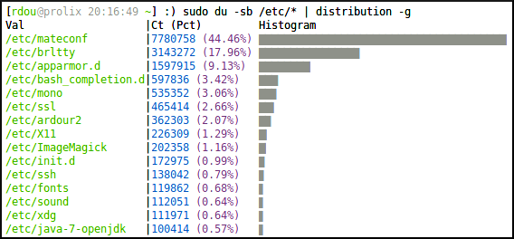
Graphing Pre-Tallied Tokens Example
===================================
Sometimes the output you have is already some keys with their counts. For
example the output of "du" or "command | uniq -c". In these cases, use the
--graph (-g) option, which skips the parsing and tokenizing of the input.
Further, you can use very short versions of the options in case you don't like
typing a lot. The default character is "+" because it creates a type of grid
system which makes it easy for the eye to trace right/left or up/down.
```
$ sudo du -sb /etc/* | distribution -w=90 -h=15 -g
Val |Ct (Pct) Histogram
/etc/mateconf |7780758 (44.60%) +++++++++++++++++++++++++++++++++++++++++++++++++
/etc/brltty |3143272 (18.02%) ++++++++++++++++++++
/etc/apparmor.d |1597915 (9.16%) ++++++++++
/etc/bash_completion.d|597836 (3.43%) ++++
/etc/mono |535352 (3.07%) ++++
/etc/ssl |465414 (2.67%) +++
/etc/ardour2 |362303 (2.08%) +++
/etc/X11 |226309 (1.30%) ++
/etc/ImageMagick |202358 (1.16%) ++
/etc/init.d |143281 (0.82%) +
/etc/ssh |138042 (0.79%) +
/etc/fonts |119862 (0.69%) +
/etc/sound |112051 (0.64%) +
/etc/xdg |111971 (0.64%) +
/etc/java-7-openjdk |100414 (0.58%) +
```
Keys in Natural Order Examples
==============================
The output is separated between STDOUT and STDERR so you can sort the resulting
histogram by values. This is useful for time series or other cases where the
keys you're graphing are in some natural order. Note how the "-v" output still
appears at the top.
```
$ cat NotServingRegionException-DateHour.txt \
| distribution -v \
| sort -n
tokens/lines examined: 1,414,196
tokens/lines matched: 1,414,196
histogram keys: 453
runtime: 1279.30ms
Val |Ct (Pct) Histogram
2012-07-13 03|38360 (2.71%) ++++++++++++++++++++++++
2012-07-28 21|18293 (1.29%) ++++++++++++
2012-07-28 23|20748 (1.47%) +++++++++++++
2012-07-29 06|15692 (1.11%) ++++++++++
2012-07-29 07|30432 (2.15%) +++++++++++++++++++
2012-07-29 08|76943 (5.44%) ++++++++++++++++++++++++++++++++++++++++++++++++
2012-07-29 09|54955 (3.89%) ++++++++++++++++++++++++++++++++++
2012-07-30 05|15652 (1.11%) ++++++++++
2012-07-30 09|40102 (2.84%) +++++++++++++++++++++++++
2012-07-30 10|21718 (1.54%) ++++++++++++++
2012-07-30 16|16041 (1.13%) ++++++++++
2012-08-01 09|22740 (1.61%) ++++++++++++++
2012-08-02 04|31851 (2.25%) ++++++++++++++++++++
2012-08-02 06|28748 (2.03%) ++++++++++++++++++
2012-08-02 07|18062 (1.28%) ++++++++++++
2012-08-02 20|23519 (1.66%) +++++++++++++++
2012-08-03 03|21587 (1.53%) ++++++++++++++
2012-08-03 08|33409 (2.36%) +++++++++++++++++++++
2012-08-03 10|15854 (1.12%) ++++++++++
2012-08-03 15|29828 (2.11%) +++++++++++++++++++
2012-08-03 16|20478 (1.45%) +++++++++++++
2012-08-03 17|39758 (2.81%) +++++++++++++++++++++++++
2012-08-03 18|19514 (1.38%) ++++++++++++
2012-08-03 19|18353 (1.30%) ++++++++++++
2012-08-03 22|18726 (1.32%) ++++++++++++
__________________
$ cat /usr/share/dict/words \
| awk '{print length($1)}' \
| distribution -c=: -w=90 -h=16 \
| sort -n
Val|Ct (Pct) Histogram
2 |182 (0.18%) :
3 |845 (0.85%) ::::
4 |3346 (3.37%) ::::::::::::::::
5 |6788 (6.84%) :::::::::::::::::::::::::::::::
6 |11278 (11.37%) ::::::::::::::::::::::::::::::::::::::::::::::::::::
7 |14787 (14.91%) :::::::::::::::::::::::::::::::::::::::::::::::::::::::::::::::::::
8 |15674 (15.81%) ::::::::::::::::::::::::::::::::::::::::::::::::::::::::::::::::::::::::
9 |14262 (14.38%) :::::::::::::::::::::::::::::::::::::::::::::::::::::::::::::::::
10|11546 (11.64%) :::::::::::::::::::::::::::::::::::::::::::::::::::::
11|8415 (8.49%) :::::::::::::::::::::::::::::::::::::::
12|5508 (5.55%) :::::::::::::::::::::::::
13|3236 (3.26%) :::::::::::::::
14|1679 (1.69%) ::::::::
15|893 (0.90%) :::::
16|382 (0.39%) ::
17|176 (0.18%) :
```
MySQL Slow Query Log Analysis Examples
======================================
You can sometimes gain interesting insights just by measuring the size of files
on your filesystem. Someone had captured slow-query-logs for every hour for
most of a day. Assuming they all compressed the same (a proper analysis would
be on uncompressed files - uncompressing them would have caused server impact -
this is good enough for illustration's sake), we can determine how much slow
query traffic appeared during a given hour of the day.
Something happened around 8am but otherwise the server seems to follow a normal
sinusoidal pattern. But note because we're only analysing the file size, it
could be that 8am had the same number of slow queries, but that the queries
themselves were larger in byte-count. Or that the queries didn't compress as
well.
Also note that we aren't seeing every histogram entry here. Always take care to
remember the tool is hiding low-frequency data from you unless you ask it to
draw uncommonly-tall histograms.
```
$ du -sb mysql-slow.log.*.gz | ~/distribution -g | sort -n
Val |Ct (Pct) Histogram
mysql-slow.log.01.gz|1426694 (5.38%) ++++++++++++++++++++
mysql-slow.log.02.gz|1499467 (5.65%) +++++++++++++++++++++
mysql-slow.log.03.gz|1840727 (6.94%) ++++++++++++++++++++++++++
mysql-slow.log.04.gz|1570131 (5.92%) ++++++++++++++++++++++
mysql-slow.log.05.gz|1439021 (5.42%) ++++++++++++++++++++
mysql-slow.log.07.gz|859939 (3.24%) ++++++++++++
mysql-slow.log.08.gz|2976177 (11.21%) ++++++++++++++++++++++++++++++++++++++++++
mysql-slow.log.09.gz|792269 (2.99%) +++++++++++
mysql-slow.log.11.gz|722148 (2.72%) ++++++++++
mysql-slow.log.12.gz|825731 (3.11%) ++++++++++++
mysql-slow.log.14.gz|1476023 (5.56%) +++++++++++++++++++++
mysql-slow.log.15.gz|2087129 (7.86%) +++++++++++++++++++++++++++++
mysql-slow.log.16.gz|1905867 (7.18%) +++++++++++++++++++++++++++
mysql-slow.log.19.gz|1314297 (4.95%) +++++++++++++++++++
mysql-slow.log.20.gz|802212 (3.02%) ++++++++++++
```
A more-proper analysis on another set of slow logs involved actually getting
the time the query ran, pulling out the date/hour portion of the timestamp, and
graphing the result.
At first blush, it might appear someone had captured logs for various hours of
one day and at 10am for several days in a row. However, note that the Pct
column shows this is only about 20% of all data, which we can also conclude
because there are 964 histogram entries, of which we're only seeing a couple
dozen. This means something happened on July 31st that caused slow queries all
day, and then 10am is a time of day when slow queries tend to happen. To test
this theory, we might re-run this with a "--height=600" (or even 900) to see
nearly all the entries to get a more precise idea of what's going on.
```
$ zcat mysql-slow.log.*.gz \
| fgrep Time: \
| cut -c 9-17 \
| ~/distribution --width=90 --verbose \
| sort -n
tokens/lines examined: 30,027
tokens/lines matched: 30,027
histogram keys: 964
runtime: 1224.58ms
Val |Ct (Pct) Histogram
120731 03|274 (0.91%) ++++++++++++++++++++++++++++++++++
120731 04|210 (0.70%) ++++++++++++++++++++++++++
120731 07|208 (0.69%) ++++++++++++++++++++++++++
120731 08|271 (0.90%) +++++++++++++++++++++++++++++++++
120731 09|403 (1.34%) +++++++++++++++++++++++++++++++++++++++++++++++++
120731 10|556 (1.85%) ++++++++++++++++++++++++++++++++++++++++++++++++++++++++++++++++++++
120731 11|421 (1.40%) +++++++++++++++++++++++++++++++++++++++++++++++++++
120731 12|293 (0.98%) ++++++++++++++++++++++++++++++++++++
120731 13|327 (1.09%) ++++++++++++++++++++++++++++++++++++++++
120731 14|318 (1.06%) +++++++++++++++++++++++++++++++++++++++
120731 15|446 (1.49%) ++++++++++++++++++++++++++++++++++++++++++++++++++++++
120731 16|397 (1.32%) ++++++++++++++++++++++++++++++++++++++++++++++++
120731 17|228 (0.76%) ++++++++++++++++++++++++++++
120801 10|515 (1.72%) +++++++++++++++++++++++++++++++++++++++++++++++++++++++++++++++
120803 10|223 (0.74%) +++++++++++++++++++++++++++
120809 10|215 (0.72%) ++++++++++++++++++++++++++
120810 10|210 (0.70%) ++++++++++++++++++++++++++
120814 10|193 (0.64%) ++++++++++++++++++++++++
120815 10|205 (0.68%) +++++++++++++++++++++++++
120816 10|207 (0.69%) +++++++++++++++++++++++++
120817 10|226 (0.75%) ++++++++++++++++++++++++++++
120819 10|197 (0.66%) ++++++++++++++++++++++++
```
A typical problem for MySQL administrators is figuring out how many slow queries
are taking how long. The slow query log can be quite verbose. Analysing it in a
visual nature can help. For example, there is a line that looks like this in the
slow query log:
```
# Query_time: 5.260353 Lock_time: 0.000052 Rows_sent: 0 Rows_examined: 2414 Rows_affected: 1108 Rows_read: 2
```
It might be useful to see how many queries ran for how long in increments of
tenths of seconds. You can grab that third field and get tenth-second
precision with a simple awk command, then graph the result.
It seems interesting that there are spikes at 3.2, 3.5, 4, 4.3, 4.5 seconds.
One hypothesis might be that those are individual queries, each warranting its
own analysis.
```
$ head -90000 mysql-slow.log.20120710 \
| fgrep Query_time: \
| awk '{print int($3 * 10)/10}' \
| ~/distribution --verbose --height=30 --char='|o' \
| sort -n
tokens/lines examined: 12,269
tokens/lines matched: 12,269
histogram keys: 481
runtime: 12.53ms
Val|Ct (Pct) Histogram
0 |1090 (8.88%) ||||||||||||||||||||||||||||||||||||||||||||||||||||||||||||||o
2 |1018 (8.30%) |||||||||||||||||||||||||||||||||||||||||||||||||||||||||o
2.1|949 (7.73%) |||||||||||||||||||||||||||||||||||||||||||||||||||||o
2.2|653 (5.32%) |||||||||||||||||||||||||||||||||||||o
2.3|552 (4.50%) |||||||||||||||||||||||||||||||o
2.4|554 (4.52%) |||||||||||||||||||||||||||||||o
2.5|473 (3.86%) ||||||||||||||||||||||||||o
2.6|423 (3.45%) ||||||||||||||||||||||||o
2.7|394 (3.21%) ||||||||||||||||||||||o
2.8|278 (2.27%) |||||||||||||||o
2.9|189 (1.54%) ||||||||||o
3 |173 (1.41%) |||||||||o
3.1|193 (1.57%) ||||||||||o
3.2|200 (1.63%) |||||||||||o
3.3|138 (1.12%) |||||||o
3.4|176 (1.43%) ||||||||||o
3.5|213 (1.74%) ||||||||||||o
3.6|157 (1.28%) ||||||||o
3.7|134 (1.09%) |||||||o
3.8|121 (0.99%) ||||||o
3.9|96 (0.78%) |||||o
4 |110 (0.90%) ||||||o
4.1|80 (0.65%) ||||o
4.2|84 (0.68%) ||||o
4.3|90 (0.73%) |||||o
4.4|76 (0.62%) ||||o
4.5|93 (0.76%) |||||o
4.6|79 (0.64%) ||||o
4.7|71 (0.58%) ||||o
5.1|70 (0.57%) |||o
```
Apache Logs Analysis Example
============================
Even if you know sed/awk/grep, the built-in tokenizing/matching can be less
verbose. Say you want to look at all the URLs in your Apache logs. People will
be doing GET /a/b/c /a/c/f q/r/s q/n/p. A and Q are the most common, so you can
tokenize on / and the latter parts of the URL will be buried, statistically.
By tokenizing and matching using the script, you may also find unexpected
common portions of the URL that don't show up in the prefix.
```
$ zcat access.log*gz \
| awk '{print $7}' \
| distribution -t=/ -h=15
Val |Ct (Pct) Histogram
Art |1839 (16.58%) +++++++++++++++++++++++++++++++++++++++++++++++++
Rendered |1596 (14.39%) ++++++++++++++++++++++++++++++++++++++++++
Blender |1499 (13.52%) ++++++++++++++++++++++++++++++++++++++++
AznRigging |760 (6.85%) ++++++++++++++++++++
Music |457 (4.12%) ++++++++++++
Ringtones |388 (3.50%) +++++++++++
CuteStance |280 (2.52%) ++++++++
Traditional |197 (1.78%) ++++++
Technology |171 (1.54%) +++++
CreativeExhaust|134 (1.21%) ++++
Fractals |127 (1.15%) ++++
robots.txt |125 (1.13%) ++++
RingtoneEP1.mp3|125 (1.13%) ++++
Poetry |108 (0.97%) +++
RingtoneEP2.mp3|95 (0.86%) +++
```
Here we had pulled apart our access logs and put them in TSV format for input
into Hive. The user agent string was in the 13th position. I wanted to just get an
overall idea of what sort of user agents were coming to the site. I'm using the
minimal argument size and my favorite "character" combo of "|o". I find it interesting
that there were only 474 unique word-based tokens in the input. Also, it's clear
that a large percentage of the visitors come with mobile devices now.
```
$ zcat weblog-2014-05.tsv.gz \
| awk -F '\t' '{print $13}' \
| distribution -t=word -m=word -c='|o' -s=m -v
tokens/lines examined: 28,062,913
tokens/lines matched: 11,507,407
histogram keys: 474
runtime: 15659.97ms
Val |Ct (Pct) Histogram
Mozilla |912852 (7.93%) ||||||||||||||||||||||||||||||||||||||||||||||||||||||||||||||||||||||||o
like |722945 (6.28%) |||||||||||||||||||||||||||||||||||||||||||||||||||||||||o
OS |611503 (5.31%) ||||||||||||||||||||||||||||||||||||||||||||||||o
AppleWebKit|605618 (5.26%) |||||||||||||||||||||||||||||||||||||||||||||||o
Gecko |535620 (4.65%) ||||||||||||||||||||||||||||||||||||||||||o
Windows |484056 (4.21%) ||||||||||||||||||||||||||||||||||||||o
NT |483085 (4.20%) ||||||||||||||||||||||||||||||||||||||o
KHTML |356730 (3.10%) ||||||||||||||||||||||||||||o
Safari |355400 (3.09%) ||||||||||||||||||||||||||||o
X |347033 (3.02%) |||||||||||||||||||||||||||o
Mac |344205 (2.99%) |||||||||||||||||||||||||||o
appversion |300816 (2.61%) |||||||||||||||||||||||o
Type |299085 (2.60%) |||||||||||||||||||||||o
Connection |299085 (2.60%) |||||||||||||||||||||||o
Mobile |282759 (2.46%) ||||||||||||||||||||||o
CPU |266837 (2.32%) |||||||||||||||||||||o
NET |247418 (2.15%) |||||||||||||||||||o
CLR |247418 (2.15%) |||||||||||||||||||o
Aspect |242566 (2.11%) |||||||||||||||||||o
Ratio |242566 (2.11%) |||||||||||||||||||o
```
And here we had a list of referrers in "referrer [count]" format. They were done one per day, but I wanted a count for January through September, so I used a shell glob to specify all those files for my 'cat'. Distribution will notice that it's getting the same key as previously and just add the new value, so the key "x1" can come in many times and we'll get the aggregate in the output. The referrers have been anonymized here since they are very specific to the company.
```
$ cat referrers-20140* | distribution -v -g=kv -s=m
tokens/lines examined: 133,564
tokens/lines matched: 31,498,986
histogram keys: 14,882
runtime: 453.45ms
Val |Ct (Pct) Histogram
x1 |24313595 (77.19%) ++++++++++++++++++++++++++++++++++++++++++++++++++++
x2 |3430278 (10.89%) ++++++++
x3 |1049996 (3.33%) +++
x4 |210083 (0.67%) +
x5 |179554 (0.57%) +
x6 |163158 (0.52%) +
x7 |129997 (0.41%) +
x8 |122725 (0.39%) +
x9 |120487 (0.38%) +
xa |109085 (0.35%) +
xb |99956 (0.32%) +
xc |92208 (0.29%) +
xd |90017 (0.29%) +
xe |79416 (0.25%) +
xf |70094 (0.22%) +
xg |58089 (0.18%) +
xh |52349 (0.17%) +
xi |37002 (0.12%) +
xj |36651 (0.12%) +
xk |32860 (0.10%) +
```
This seems a really good time to use the --logarithmic option, since that top referrer
is causing a loss of resolution on the following ones! I'll re-run this for one month.
```
$ cat referrers-201402* | distribution -v -g=kv -s=m -l
tokens/lines examined: 23,517
tokens/lines matched: 5,908,765
histogram keys: 5,888
runtime: 78.28ms
Val |Ct (Pct) Histogram
x1 |4471708 (75.68%) +++++++++++++++++++++++++++++++++++++++++++++++++++++
x2 |670703 (11.35%) ++++++++++++++++++++++++++++++++++++++++++++++
x3 |203489 (3.44%) ++++++++++++++++++++++++++++++++++++++++++
x4 |43751 (0.74%) +++++++++++++++++++++++++++++++++++++
x5 |36211 (0.61%) ++++++++++++++++++++++++++++++++++++
x6 |34589 (0.59%) ++++++++++++++++++++++++++++++++++++
x7 |31279 (0.53%) ++++++++++++++++++++++++++++++++++++
x8 |29596 (0.50%) +++++++++++++++++++++++++++++++++++
x9 |23125 (0.39%) +++++++++++++++++++++++++++++++++++
xa |21429 (0.36%) ++++++++++++++++++++++++++++++++++
xb |19670 (0.33%) ++++++++++++++++++++++++++++++++++
xc |19057 (0.32%) ++++++++++++++++++++++++++++++++++
xd |18945 (0.32%) ++++++++++++++++++++++++++++++++++
xe |18936 (0.32%) ++++++++++++++++++++++++++++++++++
xf |16015 (0.27%) +++++++++++++++++++++++++++++++++
xg |13115 (0.22%) +++++++++++++++++++++++++++++++++
xh |12067 (0.20%) ++++++++++++++++++++++++++++++++
xi |8485 (0.14%) +++++++++++++++++++++++++++++++
xj |7694 (0.13%) +++++++++++++++++++++++++++++++
xk |7199 (0.12%) +++++++++++++++++++++++++++++++
```
Graphing a Series of Numbers Example
====================================
Suppose you just have a list of integers you want to graph. For example, you've
captured a "show global status" for every second for 5 minutes, and you want to
grep out just one stat for the five-minute sample and graph it.
Or, slightly more-difficult, you want to pull out the series of numbers and
only graph the difference between each pair (as in a monotonically-increasing
counter). The ```--numonly=``` option takes care of both these cases. This option
will override any "height" and simply graph all the numbers, since there's no
frequency to dictate which values are more important to graph than others.
Therefore there's a lot of output, which is snipped in the example output that
follows. The "val" column is simply an ascending list of integers, so you can
tell where output was snipped by the jumps in those values.
```
$ grep ^Innodb_data_reads globalStatus*.txt \
| awk '{print $2}' \
| distribution --numonly=mon --char='|+'
Val|Ct (Pct) Histogram
1 |0 (0.00%) +
91 |15 (0.05%) +
92 |14 (0.04%) +
93 |30 (0.10%) |+
94 |11 (0.03%) +
95 |922 (2.93%) |||||||||||||||||||||||||||||||||||||||||||||||||||||||||+
96 |372 (1.18%) |||||||||||||||||||||||+
97 |44 (0.14%) ||+
98 |37 (0.12%) ||+
99 |110 (0.35%) ||||||+
100|18 (0.06%) |+
101|12 (0.04%) +
102|19 (0.06%) |+
103|164 (0.52%) ||||||||||+
200|62 (0.20%) |||+
201|372 (1.18%) |||||||||||||||||||||||+
202|228 (0.72%) ||||||||||||||+
203|43 (0.14%) ||+
204|917 (2.91%) ||||||||||||||||||||||||||||||||||||||||||||||||||||||||+
205|64 (0.20%) |||+
206|178 (0.57%) |||||||||||+
207|90 (0.29%) |||||+
208|90 (0.29%) |||||+
209|101 (0.32%) ||||||+
453|0 (0.00%) +
454|0 (0.00%) +
```
The Python version eschews the header and superfluous "key" as the Perl version
will probably also soon do:
```
$ cat ~/tmp/numberSeries.txt | xargs
01 05 06 09 12 22 28 32 34 30 37 44 48 54 63 70 78 82 85 88 89 89 90 92 95
$ cat ~/tmp/numberSeries.txt \
| ~/Dev/distribution/distribution.py --numonly -c='|o' -s=s
5 (0.39%) ||o
6 (0.47%) ||o
9 (0.70%) ||||o
12 (0.94%) |||||o
22 (1.71%) ||||||||||o
28 (2.18%) |||||||||||||o
32 (2.49%) |||||||||||||||o
34 (2.65%) ||||||||||||||||o
30 (2.34%) ||||||||||||||o
37 (2.88%) |||||||||||||||||o
44 (3.43%) ||||||||||||||||||||o
48 (3.74%) ||||||||||||||||||||||o
54 (4.21%) |||||||||||||||||||||||||o
63 (4.91%) |||||||||||||||||||||||||||||o
70 (5.46%) |||||||||||||||||||||||||||||||||o
78 (6.08%) ||||||||||||||||||||||||||||||||||||o
82 (6.39%) ||||||||||||||||||||||||||||||||||||||o
85 (6.63%) ||||||||||||||||||||||||||||||||||||||||o
88 (6.86%) |||||||||||||||||||||||||||||||||||||||||o
89 (6.94%) ||||||||||||||||||||||||||||||||||||||||||o
89 (6.94%) ||||||||||||||||||||||||||||||||||||||||||o
90 (7.01%) ||||||||||||||||||||||||||||||||||||||||||o
92 (7.17%) |||||||||||||||||||||||||||||||||||||||||||o
95 (7.40%) |||||||||||||||||||||||||||||||||||||||||||||o
$ cat ~/tmp/numberSeries.txt \
| ~/Dev/distribution/distribution.py --numonly=diff -c='|o' -s=s
4 (4.26%) ||||||||||||||||||o
1 (1.06%) ||||o
3 (3.19%) |||||||||||||o
3 (3.19%) |||||||||||||o
10 (10.64%) |||||||||||||||||||||||||||||||||||||||||||||o
6 (6.38%) |||||||||||||||||||||||||||o
4 (4.26%) ||||||||||||||||||o
2 (2.13%) |||||||||o
-4 (-4.26%) o
7 (7.45%) |||||||||||||||||||||||||||||||o
7 (7.45%) |||||||||||||||||||||||||||||||o
4 (4.26%) ||||||||||||||||||o
6 (6.38%) |||||||||||||||||||||||||||o
9 (9.57%) ||||||||||||||||||||||||||||||||||||||||o
7 (7.45%) |||||||||||||||||||||||||||||||o
8 (8.51%) ||||||||||||||||||||||||||||||||||||o
4 (4.26%) ||||||||||||||||||o
3 (3.19%) |||||||||||||o
3 (3.19%) |||||||||||||o
1 (1.06%) ||||o
0 (0.00%) o
1 (1.06%) ||||o
2 (2.13%) |||||||||o
3 (3.19%) |||||||||||||o
```
HDFS DU Example
===============
HDFS files are often rather large, so I first change the numeric file size to
megabytes by dividing by 1048576. I must also change it to an int value, since
distribution doesn't currently deal with non-integer counts.
Also, we are pre-parsing the du output to give us only the megabytes count and
the final entry in the filename. `awk -F /` supports that.
```
$ hdfs dfs -du /apps/hive/warehouse/aedb/hitcounts_byday/cookie_type=shopper \
| awk -F / '{print int($1/1048576) " " $8}' \
| distribution -g -c='-~' --height=20 \
| sort
Key|Ct (Pct) Histogram
dt=2014-11-15|3265438 (2.53%) ----------------------------------------------~
dt=2014-11-16|3241614 (2.51%) ----------------------------------------------~
dt=2014-11-20|2964636 (2.29%) ------------------------------------------~
dt=2014-11-21|3049912 (2.36%) -------------------------------------------~
dt=2014-11-22|3292621 (2.55%) -----------------------------------------------~
dt=2014-11-23|3319538 (2.57%) -----------------------------------------------~
dt=2014-11-24|3070654 (2.38%) -------------------------------------------~
dt=2014-11-25|3086090 (2.39%) --------------------------------------------~
dt=2014-11-27|3113888 (2.41%) --------------------------------------------~
dt=2014-11-28|3124426 (2.42%) --------------------------------------------~
dt=2014-11-29|3431859 (2.66%) -------------------------------------------------~
dt=2014-11-30|3391117 (2.62%) ------------------------------------------------~
dt=2014-12-01|3167744 (2.45%) ---------------------------------------------~
dt=2014-12-02|3134248 (2.43%) --------------------------------------------~
dt=2014-12-03|3023733 (2.34%) -------------------------------------------~
dt=2014-12-04|3022274 (2.34%) -------------------------------------------~
dt=2014-12-05|3040776 (2.35%) -------------------------------------------~
dt=2014-12-06|3054159 (2.36%) -------------------------------------------~
dt=2014-12-09|3065252 (2.37%) -------------------------------------------~
dt=2014-12-10|3316703 (2.57%) -----------------------------------------------~
```
Running Tests
=============
The `tests` directory contains sample input and output files, as well as a
script to verify expected output based on the sample inputs. To use it, first
export an environment variable called `distribution` that points to the
location of your distribution executable. The script must be run from the `tests`
directory. For example, the following will run tests against the Perl script
and then against the Python script:
cd tests/
distribution=../distribution ./runTests.sh
distribution=../distribution.py ./runTests.sh
The `runTests.sh` script takes one optional argument, `-v`. This enables
verbose mode, which prints out any differences in the stderr of the test runs,
for comparing diagnostic info.
To-Do List
==========
New features are unlikely to be added, as the existing functionality is already
arguably a superset of what's necessary. Still, there are some things that need
to be done.
* No Time::HiRes Perl module? Don't die. Much harder than it should be.
Negated by next to-do.
* Get scripts into package managers.
Porting
=======
Perl and Python are fairly common, but I'm not sure 100% of systems out there
have them. A C/C++ port would be most welcome.
If you write a port, send me a pull request so I can include it in this repo.
Port requirements: from the user's point of view, it's the exact same script.
They pass in the same options in the same way, and get the same output,
byte-for-byte if possible. This means you'll need (Perl) regexp support in your
language of choice. Also a hash map structure makes the implementation simple,
but more-efficient methods are welcome.
I imagine, in order of nice-to-haveness:
* C or C++
* Go
* Lisp
* Ocaml
* Java
* Ruby
List of known ports
-------------------
1. [go-distribution](https://github.com/bradfordboyle/go-distribution)
Authors
=======
* Tim Ellis
* Philo Vivero
* Taylor Stearns