https://stocnet.github.io/autograph/
Automatic Plotting of Many Graphs
https://stocnet.github.io/autograph/
cran graphs network plotting r
Last synced: 8 months ago
JSON representation
Automatic Plotting of Many Graphs
- Host: GitHub
- URL: https://stocnet.github.io/autograph/
- Owner: stocnet
- License: other
- Created: 2024-11-26T09:53:13.000Z (over 1 year ago)
- Default Branch: main
- Last Pushed: 2025-11-18T13:17:33.000Z (8 months ago)
- Last Synced: 2025-11-18T15:59:48.575Z (8 months ago)
- Topics: cran, graphs, network, plotting, r
- Language: HTML
- Homepage: https://stocnet.github.io/autograph/
- Size: 11.5 MB
- Stars: 1
- Watchers: 4
- Forks: 0
- Open Issues: 11
-
Metadata Files:
- Readme: README.Rmd
- Changelog: NEWS.md
- Contributing: .github/CONTRIBUTING.md
- License: LICENSE
- Code of conduct: .github/CODE_OF_CONDUCT.md
Awesome Lists containing this project
- awesome-ggplot2 - autograph
README
---
output: github_document
---
```{r, include = FALSE}
knitr::opts_chunk$set(
collapse = TRUE,
comment = "#>",
fig.path = "man/figures/README-",
out.width = "100%"
)
library(autograph)
library(patchwork)
list_functions <- function(string){
paste0("`", paste(paste0(ls("package:autograph")[grepl(string, ls("package:autograph"))], "()"), collapse = "`, `"), "`")
}
list_data <- function(string){
paste0("`", paste(paste0(ls("package:autograph")[grepl(string, ls("package:autograph"))]), collapse = "`, `"), "`")
}
```
# autograph

[](https://lifecycle.r-lib.org/articles/stages.html#maturing)


[](https://app.codecov.io/gh/stocnet/autograph?branch=main)
## About the package
This package aims to make network visualisation _easier_, _succinct_,
and _consistent_.
Visualisation is a key part of the research process,
from the initial exploration of data to the analysis of results
and the presentation of findings in publications.
However, it is often a tedious and time-consuming task.
Trying to wrangle these into a consistent style for publication or presentation
can be frustrating and requires a lot of code.
While there are a number of excellent packages for network analysis in R,
they each face several of the following challenges when it comes to visualisation:
- defaults are often not sensible for different types of networks
- customisation can sometimes be difficult
- some require multiple lines of code to even produce a graph or plot
- most require multiple lines of code to produce a graph or plot that is
styled suitable for publication or presentation
- such style code needs to be repeated every time a graph or plot is produced
if a consistent style is to be maintained
- defaults and syntax are different for different packages,
so a workflow using multiple packages must adapt to multiple syntaxes
- different visual defaults can frustrate interpretation,
and potentially invites errors when comparing plots from different packages
- some plotting methods are available for some networks or network-related
results and not others
`{autograph}` aims to solve these problems by providing automatic graph drawing
for networks in any of the `{manynet}` formats,
and automatic plotting for results from `{stocnet}` packages, including `{migraph}`, `{RSiena}`, and `{MoNAn}`, and more.
All you need to do is install the package
(loading it last will make sure its plotting methods are the default),
use `set_stocnet_theme()` (once) to set your preferred theme,
and then use `graphr()` to graph your networks,
or `plot()` to plot your results.
That's it!
## Drawing graphs
`{autograph}` includes three one-line graphing functions with sensible defaults
based on the network's properties.
First, `graphr()` is used to graph networks in any of the `{manynet}` formats.
Because it builds upon `{manynet}`, it can graph networks in any of the `{manynet}` formats, including `network`, `igraph`, `sna`, `tidygraph`, and more.
Second, it includes sensible defaults so that researchers can view their network's structure
or distribution quickly with a minimum of fuss.
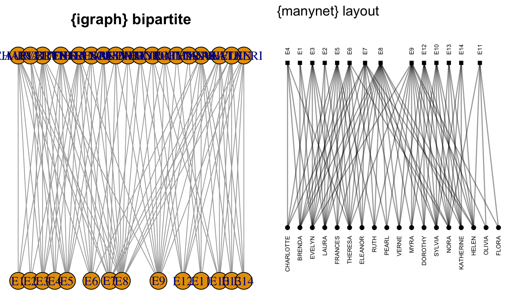
Compare the output from `{autograph}` with a similar default from `{igraph}`:
```{r layout-comparison, echo = FALSE, message=FALSE, dpi = 250, fig.height=4, fig.width=12, eval=FALSE}
library(autograph)
library(igraph)
library(gridBase)
library(grid)
par(mfrow=c(1, 2), mai = c(0,0,0.5,0))
plot(as_igraph(ison_southern_women), layout = layout_as_bipartite, main = "{igraph} bipartite")
## the last one is the current plot
plot.new() ## suggested by @Josh
vps <- baseViewports()
pushViewport(vps$figure) ## I am in the space of the autocorrelation plot
vp1 <-plotViewport(c(1.8,1,0,1)) ## create new vp with margins, you play with this values
p <- graphr(ison_southern_women) + ggtitle("{autograph} twomode") + guides(shape = "none")
print(p,vp = vp1)
```
`{igraph}` requires the bipartite layout to be specified,
has cumbersome node size defaults for all but the smallest graphs,
and labels also very often need resizing and adjustment to avoid overlap.
Getting this default plot to look good can take a lot of trial and error, and time.
By contrast, `graphr()` recognises the network as two-mode
and uses a bipartite layout by default.
It also recognises that the network contains names for the nodes and
prints them vertically so that they are legible in this layout.
Other 'clever' features include automatic node sizing and more.
### More options
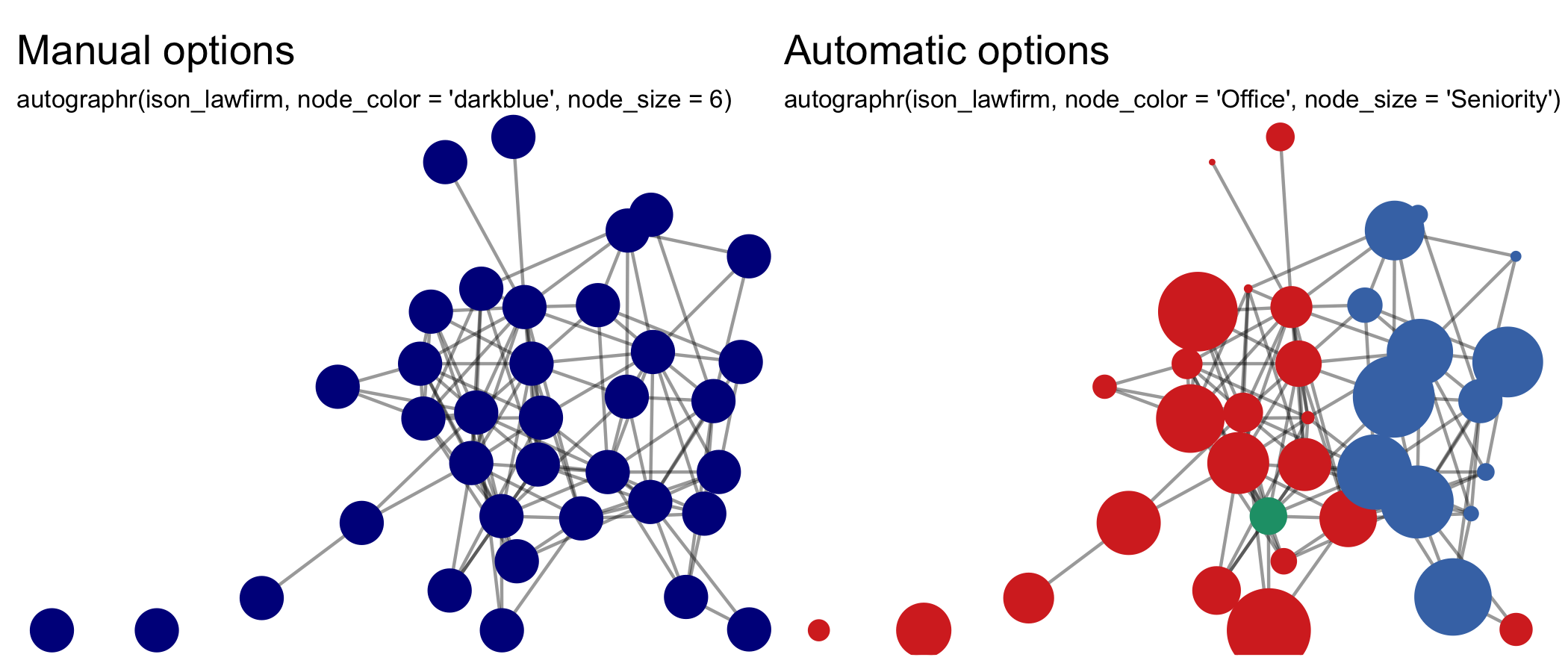
All of `graphr()`'s adjustments can be overridden, however...
Changing the size and colors of nodes and ties is as easy as
specifying the function's relevant argument with a replacement,
e.g. `node_color = "darkblue"` or `node_size = 6`,
or indicating from which attribute it should inherit this information,
e.g. `node_color = "Office"` or `node_size = "Seniority"`.
```{r more-options, echo = FALSE, message=FALSE, dpi = 300, fig.height=3, eval=FALSE}
graphr(ison_lawfirm, node_color = "darkblue", node_size = 6) +
ggtitle("Manual options",
subtitle = "graphr(ison_lawfirm, node_color = 'darkblue', node_size = 6)") +
graphr(mutate(ison_lawfirm, Seniority = Seniority/3), node_color = "Office", node_size = "Seniority") +
ggtitle("Automatic options",
subtitle = "graphr(ison_lawfirm, node_color = 'Office', node_size = 'Seniority')") &
theme(plot.subtitle = element_text(size = 8))
```
Legends are added by default when node or tie aesthetics are mapped to attributes,
but can be removed with `show_legend = FALSE`.
Since the `{autograph}` builds upon `{ggplot2}`, titles, subtitles and, for plotting, axis labels can all be added on easily,
or other elements (e.g. font size) can be tweaked for a particular output.
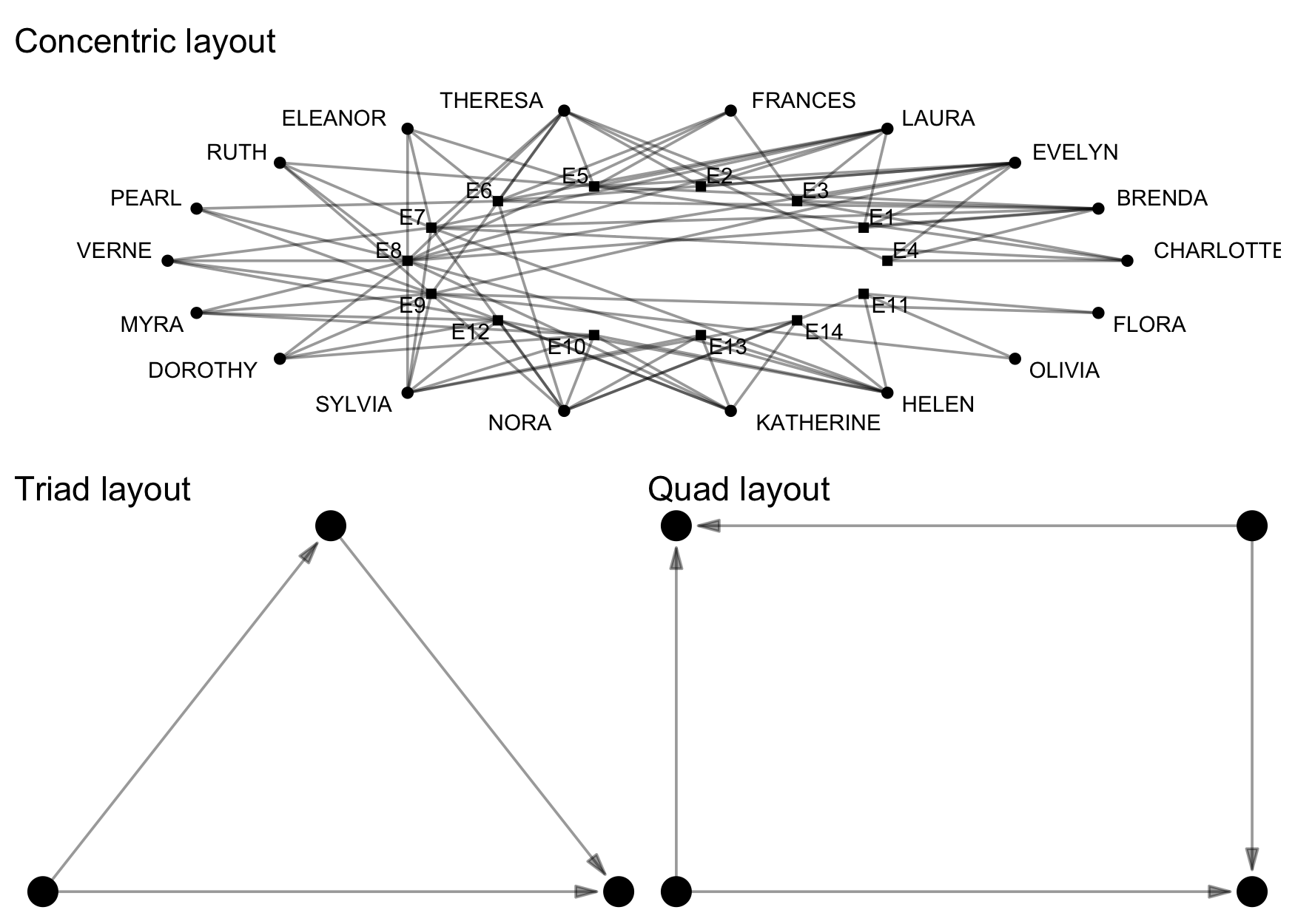
### More layouts
`graphr()` can use all the layout algorithms offered by packages such as `{igraph}`, `{ggraph}`, and `{graphlayouts}`.
`{autograph}` also offers some additional layout algorithms for
visualising partitions horizontally, vertically, or concentrically,
conforming to configurational coordinates,
or for snapping these layouts to a grid.
```{r more-layouts, echo = FALSE, message=FALSE, dpi = 250, eval=FALSE}
(graphr(ison_southern_women, layout = "concentric") + ggtitle("Concentric layout")) /
((graphr(to_unnamed(create_explicit(A-+B-+C, A-+C))) + ggtitle("Triad layout")) |
(graphr(to_unnamed(create_explicit(A-+C, A-+D, B-+C, B-+D))) + ggtitle("Quad layout")))
```
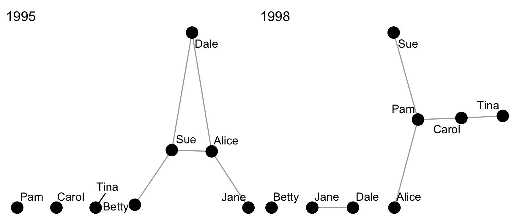
### More networks
The second graph drawing function included, `graphs()`,
is used to graph multiple networks together.
This can be useful for ego networks or network panels.
`{patchwork}` is used to help arrange individual plots together,
and is used throughout the package to help arrange plots together informatively.
```{r autographs, echo = FALSE, dpi = 250, fig.height=3, eval=FALSE}
ison_adolescents %>%
mutate_ties(wave = c(rep(1995, 5), rep(1998, 5))) %>%
to_waves(attribute = "wave", panels = c(1995, 1998)) %>%
graphs()
```
### More time
The third graph drawing function, `grapht()`,
is used to visualise dynamic networks.
It uses `{gganimate}` and `{gifski}` to create a gif that
visualises network changes over time.
It really couldn't be easier.
```{r autographd, echo = FALSE, dpi = 250, fig.height=3.5, eval=FALSE}
ison_adolescents %>%
mutate_ties(year = sample(1995:1998, 10, replace = TRUE)) %>%
to_waves(attribute = "year") %>%
grapht()
```
## Generating plots
Since network analysis involves not just drawing graphs,
`{autograph}` also provides a function for plotting results
from the analysis or modelling of those networks.
To keep things simple, all users need to remember is a single, generic function:
`plot()`.
Method dispatching takes care of the rest,
so you can concentrate on exploring and interpreting your results.
Here are some examples, using goodness-of-fit results from fitting a SAOM
in `{RSiena}` and an ERGM in `{ergm}`.
(Note that neither the data nor the model are similar;
this is just for illustrative purposes.)
```{r siena-ergm-gof, echo = FALSE, dpi = 250, fig.height=2.5, message=FALSE}
plot(siena_gof) + ggtitle("SAOM goodness-of-fit")
plot(ergm_gof) + ggtitle("ERGM goodness-of-fit")
```
### Setting a theme
Note that in the above plots, the same colour scheme and fonts were used.
They can be easily changed though.
`{autograph}` includes a number of themes that can be used to style all graphs and plots consistently.
And it is very easy to set a theme.
Just type `stocnet_theme()` to see which is the theme currently set,
and to get a list of available themes.
Then enter the chosen theme name in the function to set it.
All plots created using `{autograph}` functions will then use this theme,
until you change it again.
```{r themeset, dpi = 300, fig.height=5, fig.alt="Themed figures"}
stocnet_theme()
(plot(node_degree(ison_karateka)) +
plot(tie_betweenness(ison_karateka)))/
(plot(node_in_regular(ison_southern_women, "e")) +
plot(as_matrix(ison_southern_women),
membership = node_in_regular(ison_southern_women, "e")))
stocnet_theme("ethz")
(plot(node_degree(ison_karateka)) +
plot(tie_betweenness(ison_karateka)))/
(plot(node_in_regular(ison_southern_women, "e")) +
plot(as_matrix(ison_southern_women),
membership = node_in_regular(ison_southern_women, "e")))
```
There are a range of institutional and topical themes available,
including `r autograph:::theme_opts`,
with more on the way.
```{r theme-opts, echo=FALSE, dpi = 300, fig.height=3, fig.width=8, fig.alt="Institutional themes"}
set_stocnet_theme("iheid")
ai <- autograph:::ggpizza(ag_qualitative()) + ggtitle("IHEID") +
theme(plot.title = ggplot2::element_text(colour = ag_highlight()))
set_stocnet_theme("uzh")
au <- autograph:::ggpizza(ag_qualitative(18)) + ggtitle("UZH") +
theme(plot.title = ggplot2::element_text(colour = ag_highlight()))
set_stocnet_theme("ethz")
ae <- autograph:::ggpizza(ag_qualitative()) + ggtitle("ETHZ") +
theme(plot.title = ggplot2::element_text(colour = ag_highlight()))
set_stocnet_theme("rug")
ar <- autograph:::ggpizza(ag_qualitative()) + ggtitle("RUG") +
theme(plot.title = ggplot2::element_text(colour = ag_highlight()))
set_stocnet_theme("iast")
as <- autograph:::ggpizza(ag_qualitative()) + ggtitle("IAST") +
theme(plot.title = ggplot2::element_text(colour = ag_highlight()))
set_stocnet_theme("cmu")
ac <- autograph:::ggpizza(ag_qualitative()) + ggtitle("CMU") +
theme(plot.title = ggplot2::element_text(colour = ag_highlight()))
ai | au | ae
ar | as | ac
```
If your institution or organisation is not included and you would like it to be,
please just raise an issue on Github,
along with a link to your corporate branding or style guide if available,
and we will attempt to add it at the next opportunity.
In sum, while there is a lot of clever defaults and customisation available,
all it takes is three simple functions for your
## Installation
### Stable
The easiest way to install the latest stable version of `{autograph}` is via CRAN.
Simply open the R console and enter:
`install.packages('autograph')`
`library(autograph)` will then load the package and make the data and tutorials (see below) contained within the package available.
### Development
For the latest development version,
for slightly earlier access to new features or for testing,
you may wish to download and install the binaries from Github
or install from source locally.
The latest binary releases for all major OSes -- Windows, Mac, and Linux --
can be found [here](https://github.com/stocnet/autograph/releases/latest).
Download the appropriate binary for your operating system,
and install using an adapted version of the following commands:
- For Windows: `install.packages("~/Downloads/autograph_winOS.zip", repos = NULL)`
- For Mac: `install.packages("~/Downloads/autograph_macOS.tgz", repos = NULL)`
- For Unix: `install.packages("~/Downloads/autograph_linuxOS.tar.gz", repos = NULL)`
To install from source the latest main version of `{autograph}` from Github,
please install the `{remotes}` package from CRAN and then:
- For latest stable version:
`remotes::install_github("stocnet/autograph")`
- For latest development version:
`remotes::install_github("stocnet/autograph@develop")`
### Other sources
Those using Mac computers may also install using Macports:
`sudo port install R-autograph`
## Funding details
Development on this package has been funded by the Swiss National Science Foundation (SNSF)
[Grant Number 188976](https://data.snf.ch/grants/grant/188976):
"Power and Networks and the Rate of Change in Institutional Complexes" (PANARCHIC).