https://github.com/Boulder-Investment-Technologies/lppls
Library for fitting the LPPLS model to data.
https://github.com/Boulder-Investment-Technologies/lppls
finance python
Last synced: about 1 year ago
JSON representation
Library for fitting the LPPLS model to data.
- Host: GitHub
- URL: https://github.com/Boulder-Investment-Technologies/lppls
- Owner: Boulder-Investment-Technologies
- License: mit
- Created: 2020-04-17T16:31:23.000Z (about 6 years ago)
- Default Branch: master
- Last Pushed: 2024-08-06T15:33:11.000Z (almost 2 years ago)
- Last Synced: 2024-11-09T02:18:36.340Z (over 1 year ago)
- Topics: finance, python
- Language: Jupyter Notebook
- Homepage:
- Size: 11.4 MB
- Stars: 356
- Watchers: 25
- Forks: 111
- Open Issues: 18
-
Metadata Files:
- Readme: README.md
- License: license.txt
Awesome Lists containing this project
- awesome-quant - lppls - A Python module for fitting the [Log-Periodic Power Law Singularity (LPPLS)](https://en.wikipedia.org/wiki/Didier_Sornette#The_JLS_and_LPPLS_models) model. (Python / Indicators)
- awesome-quant - github.com/Boulder-Investment-Technologies/lppls
README


[](https://pepy.tech/project/lppls)
# Log Periodic Power Law Singularity (LPPLS) Model
`lppls` is a Python module for fitting the LPPLS model to data.
## Overview
The LPPLS model provides a flexible framework to detect bubbles and predict regime changes of a financial asset. A bubble is defined as a faster-than-exponential increase in asset price, that reflects positive feedback loop of higher return anticipations competing with negative feedback spirals of crash expectations. It models a bubble price as a power law with a finite-time singularity decorated by oscillations with a frequency increasing with time.
Try the demo:
[](https://colab.research.google.com/drive/1Qvbdj4DGNcC9Oop9mA6Vzdvsoec6k2I0?usp=sharing)
Here is the model:
```math
E[ln\ p(t)] = A + B(t_c-t)^{m}+C(t_c-t)^{m}\cos(\omega\ ln(t_c-t) - \phi)
```
where:
- $E[ln\ p(t)]$: expected log price at the date of the termination of the bubble
- $t_c$: critical time (date of termination of the bubble and transition in a new regime)
- $A$: expected log price at the peak when the end of the bubble is reached at $t_c$
- $B$: amplitude of the power law acceleration
- $C$: amplitude of the log-periodic oscillations
- $m$: degree of the super exponential growth
- $\omega$: scaling ratio of the temporal hierarchy of oscillations
- $\phi$: time scale of the oscillations
The model has three components representing a bubble. The first, $A+B(t_c-t)^{m}$, handles the hyperbolic power law. For $m$ < 1 when the price growth becomes unsustainable, and at $t_c$ the growth rate becomes infinite. The second term, $C(t_c-t)^{m}$, controls the amplitude of the oscillations. It drops to zero at the critical time $t_c$. The third term, $\cos(\omega\ ln(t_c-t) - \phi)$, models the frequency of the oscillations. They become infinite at $t_c$.
## Important links
- Official source code repo: https://github.com/Boulder-Investment-Technologies/lppls
- Download releases: https://pypi.org/project/lppls/
- Issue tracker: https://github.com/Boulder-Investment-Technologies/lppls/issues
## Installation
Dependencies
`lppls` requires:
- Python (>= 3.7)
- Matplotlib (>= 3.1.1)
- Numba (>= 0.51.2)
- NumPy (>= 1.17.0)
- Pandas (>= 0.25.0)
- SciPy (>= 1.3.0)
- Pytest (>= 6.2.1)
User installation
```
pip install -U lppls
```
## Example Use
```python
from lppls import lppls, data_loader
import numpy as np
import pandas as pd
from datetime import datetime as dt
%matplotlib inline
# read example dataset into df
data = data_loader.nasdaq_dotcom()
# convert time to ordinal
time = [pd.Timestamp.toordinal(dt.strptime(t1, '%Y-%m-%d')) for t1 in data['Date']]
# create list of observation data
price = np.log(data['Adj Close'].values)
# create observations array (expected format for LPPLS observations)
observations = np.array([time, price])
# set the max number for searches to perform before giving-up
# the literature suggests 25
MAX_SEARCHES = 25
# instantiate a new LPPLS model with the Nasdaq Dot-com bubble dataset
lppls_model = lppls.LPPLS(observations=observations)
# fit the model to the data and get back the params
tc, m, w, a, b, c, c1, c2, O, D = lppls_model.fit(MAX_SEARCHES)
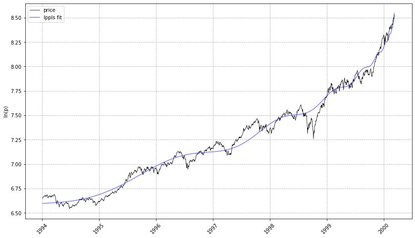
# visualize the fit
lppls_model.plot_fit()
# should give a plot like the following...
```
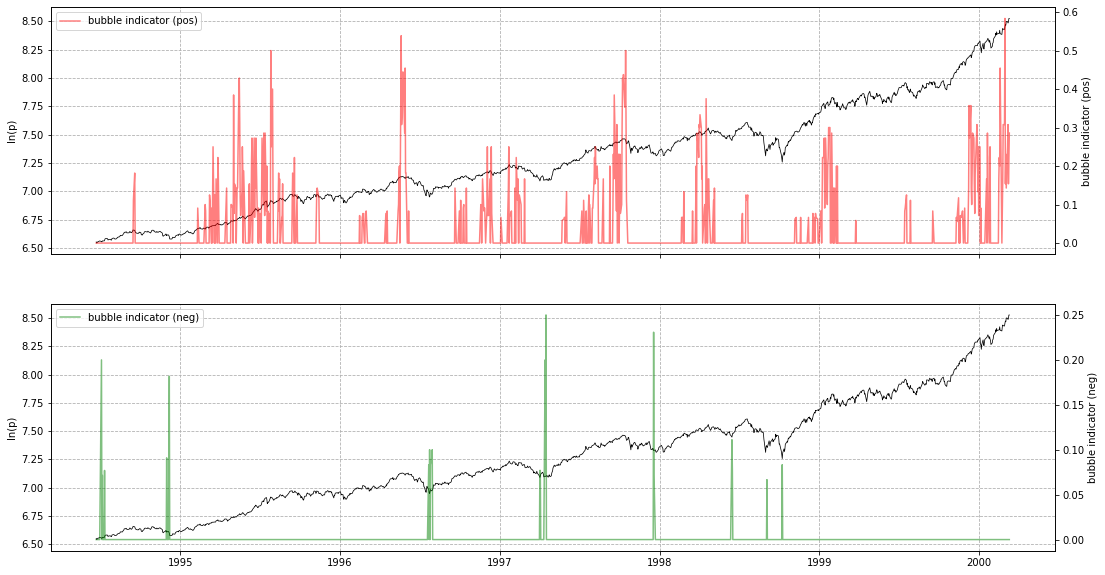
```python
# compute the confidence indicator
res = lppls_model.mp_compute_nested_fits(
workers=8,
window_size=120,
smallest_window_size=30,
outer_increment=1,
inner_increment=5,
max_searches=25,
# filter_conditions_config={} # not implemented in 0.6.x
)
lppls_model.plot_confidence_indicators(res)
# should give a plot like the following...
```
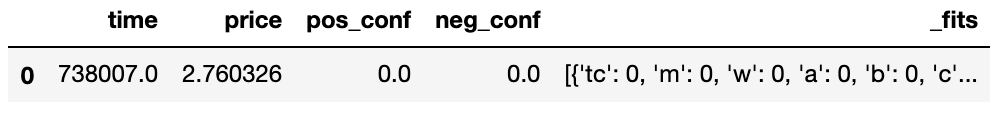
If you wish to store `res` as a pd.DataFrame, use `compute_indicators`.
Example
```python
res_df = lppls_model.compute_indicators(res)
res_df
# gives the following...
```
## Quantile Regression
Based on the work in Zhang, Zhang & Sornette 2016, quantile regression for LPPLS uses the L1 norm (sum of absolute differences) instead of the L2 norm
and applies the q-dependent loss function during calibration. Please refer to the example usage [here](https://github.com/Boulder-Investment-Technologies/lppls/blob/master/notebooks/quantile_regression.ipynb).
## Other Search Algorithms
Shu and Zhu (2019) proposed [CMA-ES](https://en.wikipedia.org/wiki/CMA-ES) for identifying the best estimation of the three non-linear parameters ($t_c$, $m$, $\omega$).
> The CMA-ES rates among the most successful evolutionary
algorithms for real-valued single-objective optimization and is typically applied to difficult
nonlinear non-convex black-box optimization problems in continuous domain and search space
dimensions between three and a hundred. Parallel computing is adopted to expedite the fitting
process drastically.
This approach has been implemented in a subclass and can be used as follows...
Thanks to @paulogonc for the code.
```python
from lppls import lppls_cmaes
lppls_model = lppls_cmaes.LPPLSCMAES(observations=observations)
tc, m, w, a, b, c, c1, c2, O, D = lppls_model.fit(max_iteration=2500, pop_size=4)
```
Performance Note: this works well for single fits but can take a long time for computing the confidence indicators. More work needs to be done to speed it up.
## References
- Filimonov, V. and Sornette, D. A Stable and Robust Calibration Scheme of the Log-Periodic Power Law Model. Physica A: Statistical Mechanics and its Applications. 2013
- Shu, M. and Zhu, W. Real-time Prediction of Bitcoin Bubble Crashes. 2019.
- Sornette, D. Why Stock Markets Crash: Critical Events in Complex Financial Systems. Princeton University Press. 2002.
- Sornette, D. and Demos, G. and Zhang, Q. and Cauwels, P. and Filimonov, V. and Zhang, Q., Real-Time Prediction and Post-Mortem Analysis of the Shanghai 2015 Stock Market Bubble and Crash (August 6, 2015). Swiss Finance Institute Research Paper No. 15-31.
- Zhang, Q., Zhang, Q., and Sornette, D. Early Warning Signals of Financial Crises with Multi-Scale Quantile Regressions of Log-Periodic Power Law Singularities. PLOS ONE. 2016. DOI:10.1371/journal.pone.0165819